rnaseq-with-replicates-limma

Published

2026-01-27

Reference & License

This tutorial is an independent reimplementation of the Bioconductor RNA-seq workflow for educational purposes.

Original workflow:
- Charity Law, Monther Alhamdoosh, Shian Su, Xueyi Dong, Luyi Tian, Gordon K. Smyth and Matthew E. Ritchie
- RNA-seq analysis is easy as 1-2-3 with limma, Glimma and edgeR

Important

本流程中，edgeR 主要負責處理原始計數資料，包括資料結構（DGEList）、低表現基因過濾（filterByExpr）以及 TMM 標準化，確保樣本之間的 library size 與組成偏差被妥善校正。

完成這些前處理後，voom 會將標準化後的計數資料轉換為 log2-CPM 並估計平均值與變異數之間的關係，進而為每一筆觀測值分配精確的權重。這個步驟使 RNA-seq 資料能夠合理地套用 limma 的線性模型與經驗貝葉斯方法，同時保留對低表現與高變異基因的適當不確定性估計。

1 分析流程圖

flowchart TD
  A[Raw counts] --> B[edgeR preprocessing]
  B --> C[TMM normalization]
  C --> D[Exploration and QC]
  D --> E[Design matrix]
  E --> F[voom transformation]
  F --> G[Linear modeling]
  G --> H[Differential expression]
  H --> I[Visualization and interpretation]

2 下載範例資料

以小鼠乳腺 RNA 定序資料為範例，先下載之後解壓縮

url <- "https://www.ncbi.nlm.nih.gov/geo/download/?acc=GSE63310&format=file"
utils::download.file(url, destfile="data/GSE63310_RAW.tar", mode="wb") 
utils::untar("data/GSE63310_RAW.tar", exdir = "./data")
files <- c("GSM1545535_10_6_5_11.txt", "GSM1545536_9_6_5_11.txt", "GSM1545538_purep53.txt",
  "GSM1545539_JMS8-2.txt", "GSM1545540_JMS8-3.txt", "GSM1545541_JMS8-4.txt",
  "GSM1545542_JMS8-5.txt", "GSM1545544_JMS9-P7c.txt", "GSM1545545_JMS9-P8c.txt")
files_path <- paste0("data/", files)
for(i in paste(files_path, ".gz", sep=""))
  R.utils::gunzip(i, overwrite=TRUE)

txt 中的資料為 EntrezID, GeneLength 與 Count，如下:

EntrezID    GeneLength  Count
497097  3634    1
100503874   3259    0
100038431   1634    0
19888   9747    0
20671   3130    1

3 讀取資料

使用 readDGE 可以直接讀取多個 txt 檔，files_path 為檔案位置的 list

library(limma)
library(Glimma)
library(edgeR)
library(Mus.musculus)

files_path
x <- readDGE(files_path, columns=c(1,3))
class(x)
dim(x)

[1] "data/GSM1545535_10_6_5_11.txt" "data/GSM1545536_9_6_5_11.txt"  "data/GSM1545538_purep53.txt"   "data/GSM1545539_JMS8-2.txt"   
[5] "data/GSM1545540_JMS8-3.txt"    "data/GSM1545541_JMS8-4.txt"    "data/GSM1545542_JMS8-5.txt"    "data/GSM1545544_JMS9-P7c.txt" 
[9] "data/GSM1545545_JMS9-P8c.txt" 
[1] "DGEList"
attr(,"package")
[1] "edgeR"
[1] 27179     9

4 創建 DGEList 物件

首先簡化名稱

samplenames <- substring(colnames(x), 17, nchar(colnames(x)))
colnames(x) <- samplenames

samplenames

[1] "10_6_5_11" "9_6_5_11"  "purep53"   "JMS8-2"    "JMS8-3"    "JMS8-4"    "JMS8-5"    "JMS9-P7c"  "JMS9-P8c"

4.1 樣本資訊(samples)

Important

通常此步驟建議用 excel 或 csv 等檔案直接匯入樣本的 metadata

group <- as.factor(c("LP", "ML", "Basal", "Basal", "ML", "LP", "Basal", "ML", "LP"))
x$samples$group <- group

lane <- as.factor(rep(c("L004","L006","L008"), c(3,4,2)))
x$samples$lane <- lane

x$samples

                                  files group lib.size norm.factors lane
10_6_5_11 data/GSM1545535_10_6_5_11.txt    LP 32863052            1 L004
9_6_5_11   data/GSM1545536_9_6_5_11.txt    ML 35335491            1 L004
purep53     data/GSM1545538_purep53.txt Basal 57160817            1 L004
JMS8-2       data/GSM1545539_JMS8-2.txt Basal 51368625            1 L006
JMS8-3       data/GSM1545540_JMS8-3.txt    ML 75795034            1 L006
JMS8-4       data/GSM1545541_JMS8-4.txt    LP 60517657            1 L006
JMS8-5       data/GSM1545542_JMS8-5.txt Basal 55086324            1 L006
JMS9-P7c   data/GSM1545544_JMS9-P7c.txt    ML 21311068            1 L008
JMS9-P8c   data/GSM1545545_JMS9-P8c.txt    LP 19958838            1 L008

4.2 準備基因對照(genes)

需要準備基因層級資訊，可以使用 biomaRt 調出所需資料

geneid <- rownames(x)
genes <- biomaRt::select(Mus.musculus, keys=geneid, columns=c("SYMBOL", "TXCHROM"), 
                         keytype="ENTREZID")
head(genes)

'select()' returned 1:many mapping between keys and columns
   ENTREZID  SYMBOL TXCHROM
1    497097    Xkr4    chr1
2 100503874 Gm19938    <NA>
3 100038431 Gm10568    <NA>
4     19888     Rp1    chr1
5     20671   Sox17    chr1
6     27395  Mrpl15    chr1

Important

必須確認是否有重複資訊，若有要處理，目前先簡化只取第一個!

genes <- genes[!duplicated(genes$ENTREZID),]
x$genes <- genes
x

An object of class "DGEList"
$samples
                                  files group lib.size norm.factors lane
10_6_5_11 data/GSM1545535_10_6_5_11.txt    LP 32863052            1 L004
9_6_5_11   data/GSM1545536_9_6_5_11.txt    ML 35335491            1 L004
purep53     data/GSM1545538_purep53.txt Basal 57160817            1 L004
JMS8-2       data/GSM1545539_JMS8-2.txt Basal 51368625            1 L006
JMS8-3       data/GSM1545540_JMS8-3.txt    ML 75795034            1 L006
JMS8-4       data/GSM1545541_JMS8-4.txt    LP 60517657            1 L006
JMS8-5       data/GSM1545542_JMS8-5.txt Basal 55086324            1 L006
JMS9-P7c   data/GSM1545544_JMS9-P7c.txt    ML 21311068            1 L008
JMS9-P8c   data/GSM1545545_JMS9-P8c.txt    LP 19958838            1 L008

$counts
           Samples
Tags        10_6_5_11 9_6_5_11 purep53 JMS8-2 JMS8-3 JMS8-4 JMS8-5 JMS9-P7c JMS9-P8c
  497097            1        2     342    526      3      3    535        2        0
  100503874         0        0       5      6      0      0      5        0        0
  100038431         0        0       0      0      0      0      1        0        0
  19888             0        1       0      0     17      2      0        1        0
  20671             1        1      76     40     33     14     98       18        8
27174 more rows ...

$genes
   ENTREZID  SYMBOL TXCHROM
1    497097    Xkr4    chr1
2 100503874 Gm19938    <NA>
3 100038431 Gm10568    <NA>
4     19888     Rp1    chr1
5     20671   Sox17    chr1
27174 more rows ...

Important

以上是完整的 DGEList 物件 所需的資料，包含 samples, counts and genes

5 前處理

5.1 取 CPM

cpm <- cpm(x)
lcpm <- cpm(x, log=TRUE)

L <- mean(x$samples$lib.size) * 1e-6
M <- median(x$samples$lib.size) * 1e-6
c(L, M)

[1] 45.48855 51.36862

summary(lcpm)

 5535_10_6_5_11    5536_9_6_5_11      5538_purep53       5539_JMS8-2       5540_JMS8-3       5541_JMS8-4       5542_JMS8-5      
 Min.   :-4.5074   Min.   :-4.5074   Min.   :-4.50743   Min.   :-4.5074   Min.   :-4.5074   Min.   :-4.5074   Min.   :-4.50743  
 1st Qu.:-4.5074   1st Qu.:-4.5074   1st Qu.:-4.50743   1st Qu.:-4.5074   1st Qu.:-4.5074   1st Qu.:-4.5074   1st Qu.:-4.50743  
 Median :-0.6847   Median :-0.3589   Median :-0.09513   Median :-0.0901   Median :-0.4281   Median :-0.4064   Median :-0.07152  
 Mean   : 0.1714   Mean   : 0.3312   Mean   : 0.43559   Mean   : 0.4089   Mean   : 0.3225   Mean   : 0.2529   Mean   : 0.40428  
 3rd Qu.: 4.2913   3rd Qu.: 4.5601   3rd Qu.: 4.60081   3rd Qu.: 4.5475   3rd Qu.: 4.5772   3rd Qu.: 4.3199   3rd Qu.: 4.42513  
 Max.   :14.7632   Max.   :13.4952   Max.   :12.95700   Max.   :12.8513   Max.   :12.9578   Max.   :14.8520   Max.   :13.19491  
 5544_JMS9-P7c     5545_JMS9-P8c    
 Min.   :-4.5074   Min.   :-4.5074  
 1st Qu.:-4.5074   1st Qu.:-4.5074  
 Median :-0.1704   Median :-0.3300  
 Mean   : 0.3708   Mean   : 0.2749  
 3rd Qu.: 4.6031   3rd Qu.: 4.4355  
 Max.   :12.9413   Max.   :14.0102

5.2 移除低表現基因

keep.exprs <- filterByExpr(x, group=group)
x <- x[keep.exprs,, keep.lib.sizes=FALSE]
dim(x)

[1] 16624     9

5.3 繪圖

lcpm.cutoff <- log2(10/M + 2/L)
library(RColorBrewer)
nsamples <- ncol(x)
col <- brewer.pal(nsamples, "Paired")

png(filename = "./images/filter_cpm.png", width = 2000, height = 1000, res = 200)
par(mfrow=c(1,2))
plot(density(lcpm[,1]), col=col[1], lwd=2, ylim=c(0,0.26), las=2, main="", xlab="")
title(main="A. Raw data", xlab="Log-cpm")
abline(v=lcpm.cutoff, lty=3)
for (i in 2:nsamples){
den <- density(lcpm[,i])
lines(den$x, den$y, col=col[i], lwd=2)
}
legend("topright", samplenames, text.col=col, bty="n")
lcpm <- cpm(x, log=TRUE)
plot(density(lcpm[,1]), col=col[1], lwd=2, ylim=c(0,0.26), las=2, main="", xlab="")
title(main="B. Filtered data", xlab="Log-cpm")
abline(v=lcpm.cutoff, lty=3)
for (i in 2:nsamples){
den <- density(lcpm[,i])
lines(den$x, den$y, col=col[i], lwd=2)
}
legend("topright", samplenames, text.col=col, bty="n")
dev.off()
par(mfrow = c(1,1))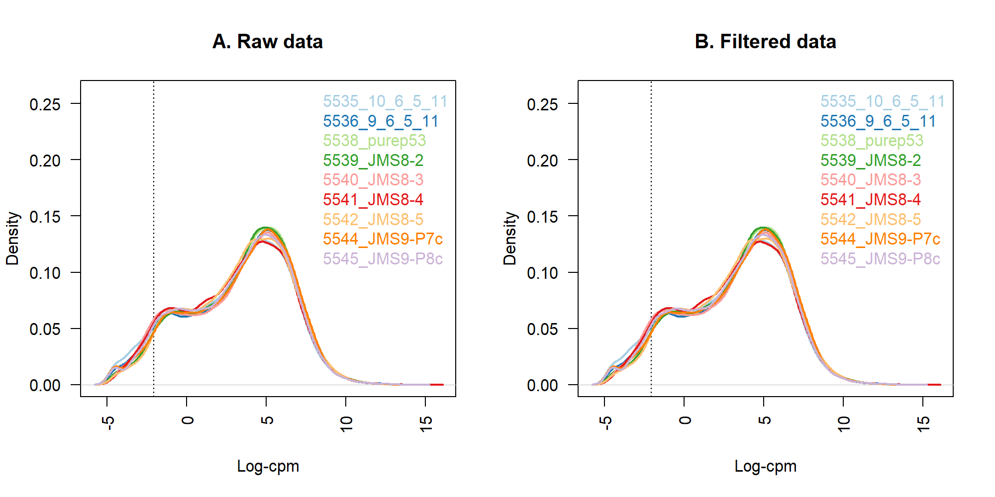

5.4 TMM 標準化

x <- calcNormFactors(x, method = "TMM")
x$samples$norm.factors

# create toy data
x2 <- x
x2$samples$norm.factors <- 1
x2$counts[,1] <- ceiling(x2$counts[,1]*0.05)
x2$counts[,2] <- x2$counts[,2]*5

# plot setting
png(filename = "./images/tmm_boxplot.png", width = 2000, height = 1000, res = 200)
par(mfrow=c(1,2))

# boxplot before TMM 
lcpm <- cpm(x2, log=TRUE)
boxplot(lcpm, las=2, col=col, main="")
title(main="A. Example: Unnormalised data",ylab="Log-cpm")

# perform TMM
x2 <- calcNormFactors(x2)  
x2$samples$norm.factors

# boxplot after TMM 
lcpm <- cpm(x2, log=TRUE)
boxplot(lcpm, las=2, col=col, main="")
title(main="B. Example: Normalised data",ylab="Log-cpm")

# plot setting
dev.off()
par(mfrow = c(1,1))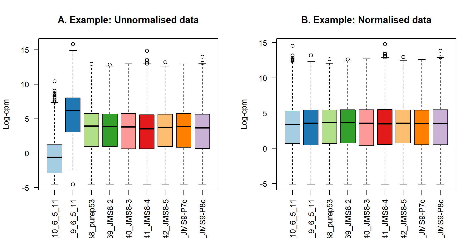

5.5 cluster 分析

png(filename = "./images/MDS.png", width = 2000, height = 1000, res = 200)
lcpm <- cpm(x, log=TRUE)
par(mfrow=c(1,2))
col.group <- group
levels(col.group) <-  brewer.pal(nlevels(col.group), "Set1")
col.group <- as.character(col.group)
col.lane <- lane
levels(col.lane) <-  brewer.pal(nlevels(col.lane), "Set2")
col.lane <- as.character(col.lane)
plotMDS(lcpm, labels=group, col=col.group)
title(main="A. Sample groups")
plotMDS(lcpm, labels=lane, col=col.lane, dim=c(3,4))
title(main="B. Sequencing lanes")
dev.off()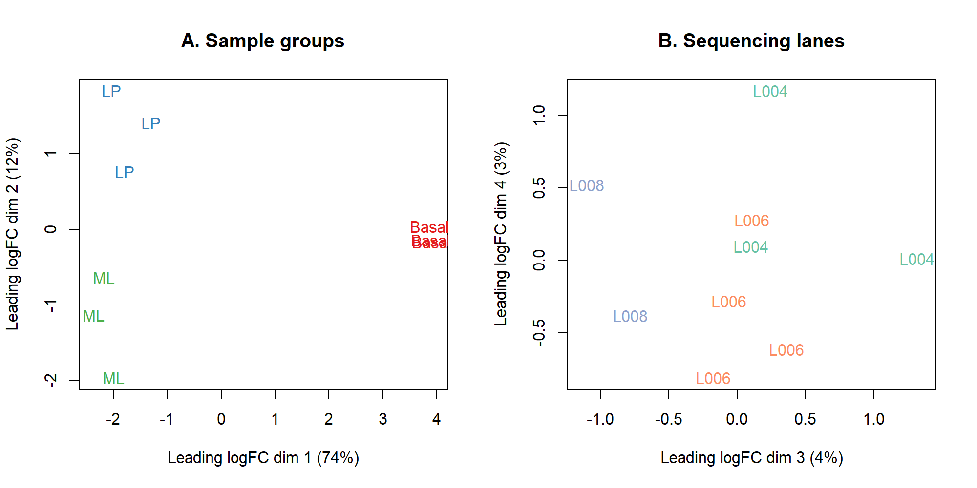

glMDSPlot(lcpm, labels=paste(group, lane, sep="_"), 
          groups=x$samples[,c(2,5)], launch=TRUE)

6 DE 分析

6.1 建立 design 矩陣

design <- model.matrix(~0+group+lane)
colnames(design) <- gsub("group", "", colnames(design))
design

  Basal LP ML laneL006 laneL008
1     0  1  0        0        0
2     0  0  1        0        0
3     1  0  0        0        0
4     1  0  0        1        0
5     0  0  1        1        0
6     0  1  0        1        0
7     1  0  0        1        0
8     0  0  1        0        1
9     0  1  0        0        1
attr(,"assign")
[1] 1 1 1 2 2
attr(,"contrasts")
attr(,"contrasts")$group
[1] "contr.treatment"

attr(,"contrasts")$lane
[1] "contr.treatment"

6.2 建立比較矩陣

contr.matrix <- makeContrasts(
   BasalvsLP = Basal-LP, 
   BasalvsML = Basal - ML, 
   LPvsML = LP - ML, 
   levels = colnames(design))
contr.matrix

          Contrasts
Levels     BasalvsLP BasalvsML LPvsML
  Basal            1         1      0
  LP              -1         0      1
  ML               0        -1     -1
  laneL006         0         0      0
  laneL008         0         0      0

6.3 voom

png(filename = "./images/voom.png", width = 2000, height = 1000, res = 200)
par(mfrow=c(1,2))
v <- voom(x, design, plot=TRUE)
v

vfit <- lmFit(v, design)
vfit <- contrasts.fit(vfit, contrasts=contr.matrix)
efit <- eBayes(vfit)
plotSA(efit, main="Final model: Mean-variance trend")
dev.off()
par(mfrow=c(1,1))

An object of class "EList"
$genes
  ENTREZID SYMBOL TXCHROM
1   497097   Xkr4    chr1
5    20671  Sox17    chr1
6    27395 Mrpl15    chr1
7    18777 Lypla1    chr1
9    21399  Tcea1    chr1
16619 more rows ...

$targets
                                       files group lib.size norm.factors lane
5535_10_6_5_11 data/GSM1545535_10_6_5_11.txt    LP 29387429    0.8943956 L004
5536_9_6_5_11   data/GSM1545536_9_6_5_11.txt    ML 36212498    1.0250186 L004
5538_purep53     data/GSM1545538_purep53.txt Basal 59771061    1.0459005 L004
5539_JMS8-2       data/GSM1545539_JMS8-2.txt Basal 53711278    1.0458455 L006
5540_JMS8-3       data/GSM1545540_JMS8-3.txt    ML 77015912    1.0162707 L006
5541_JMS8-4       data/GSM1545541_JMS8-4.txt    LP 55769890    0.9217132 L006
5542_JMS8-5       data/GSM1545542_JMS8-5.txt Basal 54863512    0.9961959 L006
5544_JMS9-P7c   data/GSM1545544_JMS9-P7c.txt    ML 23139691    1.0861026 L008
5545_JMS9-P8c   data/GSM1545545_JMS9-P8c.txt    LP 19634459    0.9839203 L008

$E
        Samples
Tags     5535_10_6_5_11 5536_9_6_5_11 5538_purep53 5539_JMS8-2 5540_JMS8-3 5541_JMS8-4 5542_JMS8-5 5544_JMS9-P7c 5545_JMS9-P8c
  497097      -4.292165     -3.856488    2.5185849   3.2931366   -4.459730   -3.994060   3.2869677    -3.2103696     -5.295316
  20671       -4.292165     -4.593453    0.3560126  -0.4073032   -1.200995   -1.943434   0.8442767    -0.3228444     -1.207853
  27395        3.876089      4.413107    4.5170045   4.5617546    4.344401    3.786363   3.8990635     4.3396075      4.124644
  18777        4.708774      5.571872    5.3964008   5.1623650    5.649355    5.081611   5.0602470     5.7513694      5.142436
  21399        4.785541      4.754537    5.3703795   5.1220551    4.869586    4.943840   5.1384776     5.0308985      4.979644
16619 more rows ...

$weights
          [,1]      [,2]      [,3]      [,4]      [,5]      [,6]      [,7]      [,8]      [,9]
[1,]  1.079413  1.332986 19.826915 20.273253  1.993686  1.395853 20.494977  1.107780  1.079413
[2,]  1.170357  1.456380  4.804866  8.660025  3.612508  2.626870  8.760149  3.211473  2.541942
[3,] 20.219073 25.573792 30.434759 28.528310 31.352260 25.743247 28.722497 21.200072 16.657930
[4,] 26.947557 32.505933 33.583128 33.232125 34.231754 32.354158 33.334340 30.348630 24.259801
[5,] 26.610864 28.501638 33.645479 33.206374 33.573492 31.996623 33.308490 25.171513 23.573305
16619 more rows ...

$design
  Basal LP ML laneL006 laneL008
1     0  1  0        0        0
2     0  0  1        0        0
3     1  0  0        0        0
4     1  0  0        1        0
5     0  0  1        1        0
6     0  1  0        1        0
7     1  0  0        1        0
8     0  0  1        0        1
9     0  1  0        0        1
attr(,"assign")
[1] 1 1 1 2 2
attr(,"contrasts")
attr(,"contrasts")$group
[1] "contr.treatment"

attr(,"contrasts")$lane
[1] "contr.treatment"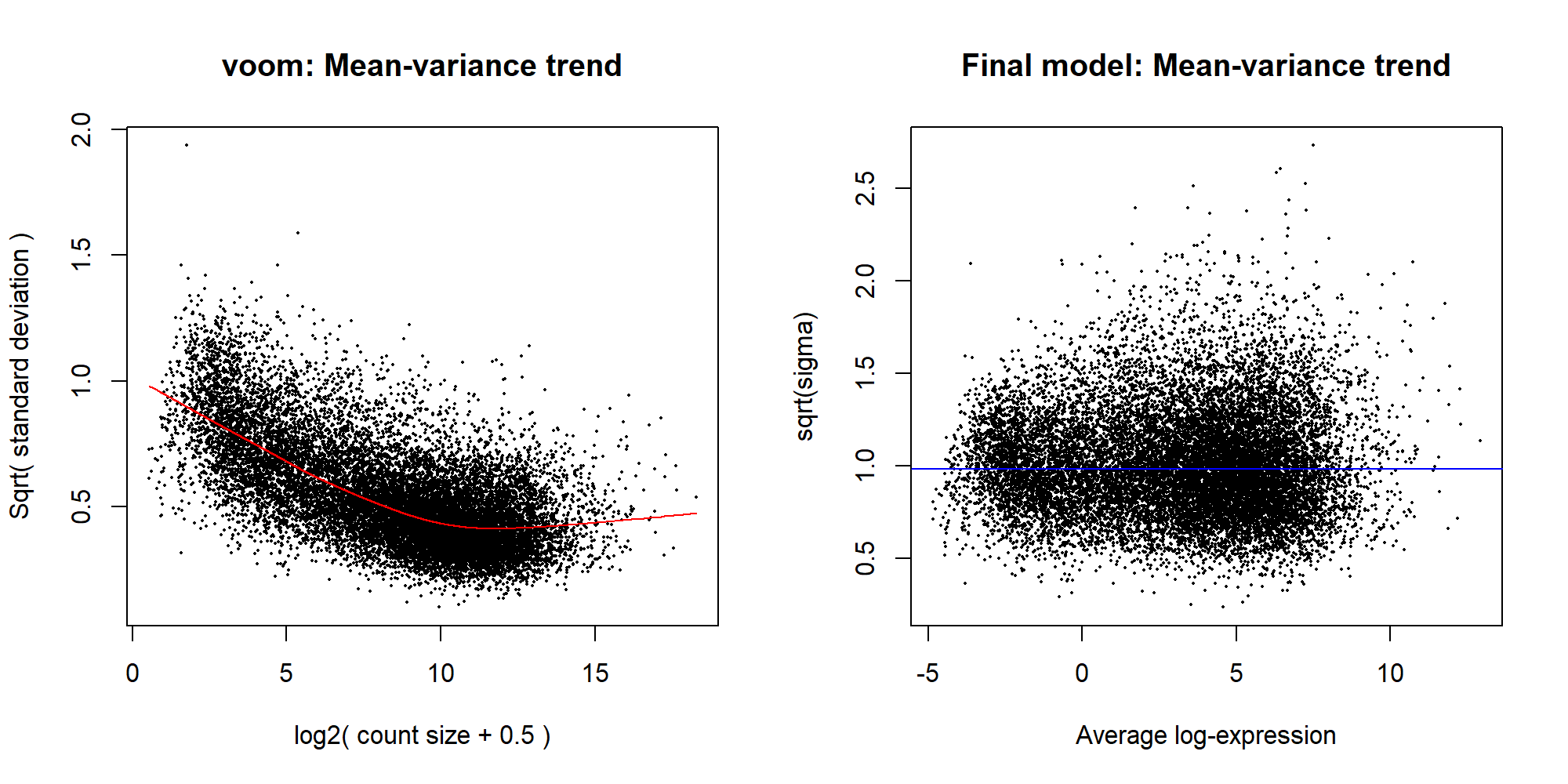

6.4 結果

summary(decideTests(efit))

       BasalvsLP BasalvsML LPvsML
Down        4648      4927   3135
NotSig      7113      7026  10972
Up          4863      4671   2517

tfit <- treat(vfit, lfc=1)
dt <- decideTests(tfit)
summary(dt)

       BasalvsLP BasalvsML LPvsML
Down        1632      1777    224
NotSig     12976     12790  16210
Up          2016      2057    190

de.common <- which(dt[,1]!=0 & dt[,2]!=0)
length(de.common)

head(tfit$genes$SYMBOL[de.common], n=20)
png(filename = "./images/venn.png", width = 1500, height = 1200, res = 200)
vennDiagram(dt[,1:2], circle.col=c("turquoise", "salmon"))
dev.off()

write.fit(tfit, dt, file="results/results.txt")

[1] 2784
 [1] "Xkr4"          "Rgs20"         "Cpa6"          "A830018L16Rik" "Sulf1"         "Eya1"          "Msc"           "Sbspon"       
 [9] "Pi15"          "Crispld1"      "Kcnq5"         "Rims1"         "Khdrbs2"       "Ptpn18"        "Prss39"        "Arhgef4"      
[17] "Cnga3"         "Cracdl"        "Aff3"          "Npas2"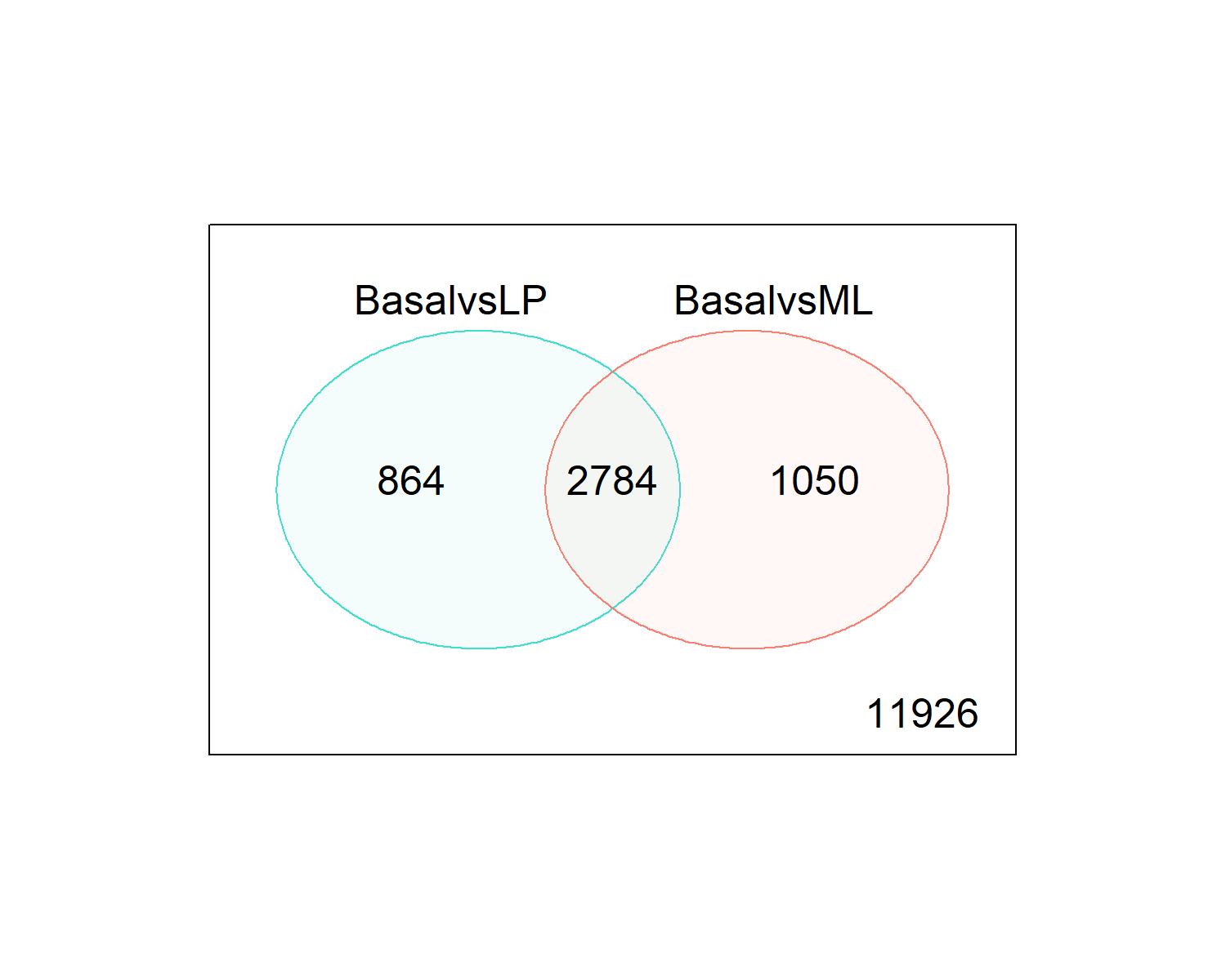

basal.vs.lp <- topTreat(tfit, coef=1, n=Inf)
basal.vs.ml <- topTreat(tfit, coef=2, n=Inf)
head(basal.vs.lp)

       ENTREZID SYMBOL TXCHROM     logFC  AveExpr         t      P.Value    adj.P.Val
12759     12759    Clu   chr14 -5.455444 8.856581 -33.55508 1.723731e-10 1.707586e-06
53624     53624  Cldn7   chr11 -5.527356 6.295437 -31.97515 2.576972e-10 1.707586e-06
242505   242505  Rasef    chr4 -5.935249 5.118259 -31.33407 3.081544e-10 1.707586e-06
67451     67451   Pkp2   chr16 -5.738665 4.419170 -29.85616 4.575686e-10 1.739242e-06
228543   228543   Rhov    chr2 -6.264208 5.485314 -29.07484 5.782844e-10 1.739242e-06
70350     70350  Basp1   chr15 -6.084738 5.247023 -28.26649 7.267694e-10 1.739242e-06

6.5 MA plot

png("images/MA-plot.png")
plotMD(tfit, column=1, status=dt[,1], main=colnames(tfit)[1], 
       xlim=c(-8,13))
dev.off()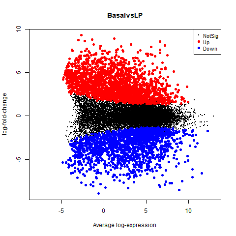

glMDPlot(tfit, coef=1, status=dt, main=colnames(tfit)[1],
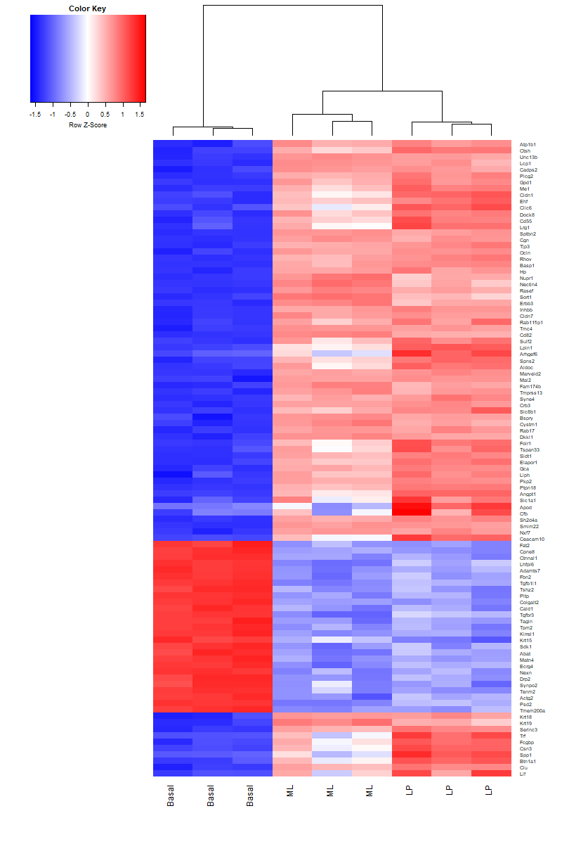
         side.main="ENTREZID", counts=lcpm, groups=group, launch=TRUE)

6.6 heatmap

library(gplots)
basal.vs.lp.topgenes <- basal.vs.lp$ENTREZID[1:100]
i <- which(v$genes$ENTREZID %in% basal.vs.lp.topgenes)
mycol <- colorpanel(1000,"blue","white","red")
png("images/heatmap.png", width = 800 ,height = 1200)
heatmap.2(lcpm[i,], scale="row",
   labRow=v$genes$SYMBOL[i], labCol=group, 
   col=mycol, trace="none", density.info="none", 
   margin=c(8,6), lhei=c(2,10), dendrogram="column")
dev.off()