library(dplyr)
library(tidyr)
library(purrr)
library(survival)
library(survminer)
library(timeROC)使用 R 做存活分析
1 基本介紹
存活分析(survival analysis)是一類用於分析「事件發生時間」資料的統計方法,廣泛應用於臨床研究、生物醫學與流行病學領域。此類資料的核心特徵在於,研究對象在追蹤期間可能尚未發生事件(例如死亡、疾病復發或失敗),因此需要同時處理「事件時間」與「截尾(censoring)」資訊。
TipReference
以下分析流程與範例內容參考 UVA HSL – BIMS 8382: Research & Data Courses / Workshops 之教學素材進行整理與改寫;完整來源與授權資訊請參考頁尾說明。
2 需求套件
首先匯入需要的套件:
3 讀取資料
讀取 survival 套件內建資料集 lung
lung_df <- as_tibble(lung)
head(lung_df)| inst | time | status | age | sex | ph.ecog | ph.karno | pat.karno | meal.cal | wt.loss |
|---|---|---|---|---|---|---|---|---|---|
| 3 | 306 | 2 | 74 | 1 | 1 | 90 | 100 | 1175 | NA |
| 3 | 455 | 2 | 68 | 1 | 0 | 90 | 90 | 1225 | 15 |
| 3 | 1010 | 1 | 56 | 1 | 0 | 90 | 90 | NA | 15 |
| 5 | 210 | 2 | 57 | 1 | 1 | 90 | 60 | 1150 | 11 |
| 1 | 883 | 2 | 60 | 1 | 0 | 100 | 90 | NA | 0 |
| 12 | 1022 | 1 | 74 | 1 | 1 | 50 | 80 | 513 | 0 |
4 擬合生存曲線
以性別來擬合生存曲線
sfit <- survfit(Surv(time, status)~sex, data=lung)
sfit
summary(sfit)
Call: survfit(formula = Surv(time, status) ~ sex, data = lung)
n events median 0.95LCL 0.95UCL
sex=1 138 112 270 212 310
sex=2 90 53 426 348 550
Call: survfit(formula = Surv(time, status) ~ sex, data = lung)
sex=1
time n.risk n.event survival std.err lower 95% CI upper 95% CI
11 138 3 0.9783 0.0124 0.9542 1.000
12 135 1 0.9710 0.0143 0.9434 0.999
13 134 2 0.9565 0.0174 0.9231 0.991
15 132 1 0.9493 0.0187 0.9134 0.987
26 131 1 0.9420 0.0199 0.9038 0.982
30 130 1 0.9348 0.0210 0.8945 0.977
31 129 1 0.9275 0.0221 0.8853 0.972
53 128 2 0.9130 0.0240 0.8672 0.961
54 126 1 0.9058 0.0249 0.8583 0.956
59 125 1 0.8986 0.0257 0.8496 0.950
60 124 1 0.8913 0.0265 0.8409 0.945
.......................<Skip>.........................可以對 summary()函數 指定結果中顯示的時間範圍
summary(sfit, times=seq(0, 1000, 100))Call: survfit(formula = Surv(time, status) ~ sex, data = lung)
sex=1
time n.risk n.event survival std.err lower 95% CI upper 95% CI
0 138 0 1.0000 0.0000 1.0000 1.000
100 114 24 0.8261 0.0323 0.7652 0.892
200 78 30 0.6073 0.0417 0.5309 0.695
300 49 20 0.4411 0.0439 0.3629 0.536
400 31 15 0.2977 0.0425 0.2250 0.394
500 20 7 0.2232 0.0402 0.1569 0.318
600 13 7 0.1451 0.0353 0.0900 0.234
700 8 5 0.0893 0.0293 0.0470 0.170
800 6 2 0.0670 0.0259 0.0314 0.143
900 2 2 0.0357 0.0216 0.0109 0.117
1000 2 0 0.0357 0.0216 0.0109 0.117
sex=2
time n.risk n.event survival std.err lower 95% CI upper 95% CI
0 90 0 1.0000 0.0000 1.0000 1.000
100 82 7 0.9221 0.0283 0.8683 0.979
200 66 11 0.7946 0.0432 0.7142 0.884
300 43 9 0.6742 0.0523 0.5791 0.785
400 26 10 0.5089 0.0603 0.4035 0.642
500 21 5 0.4110 0.0626 0.3050 0.554
600 11 3 0.3433 0.0634 0.2390 0.493
700 8 3 0.2496 0.0652 0.1496 0.417
800 2 5 0.0832 0.0499 0.0257 0.270
900 1 0 0.0832 0.0499 0.0257 0.2705 繪製 Kaplan-Meier plot
sfit <- survfit(Surv(time, status)~sex, data=lung)

png("./images/KM_simple.png", width = 800, height = 600, res = 120)
plot(sfit)
dev.off()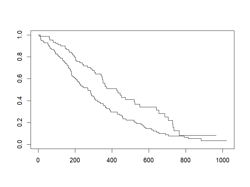
可以用 survminer 繪製精美圖表
survminer::ggsurvplot(sfit)
ggsave("./images/KM_pretty.png")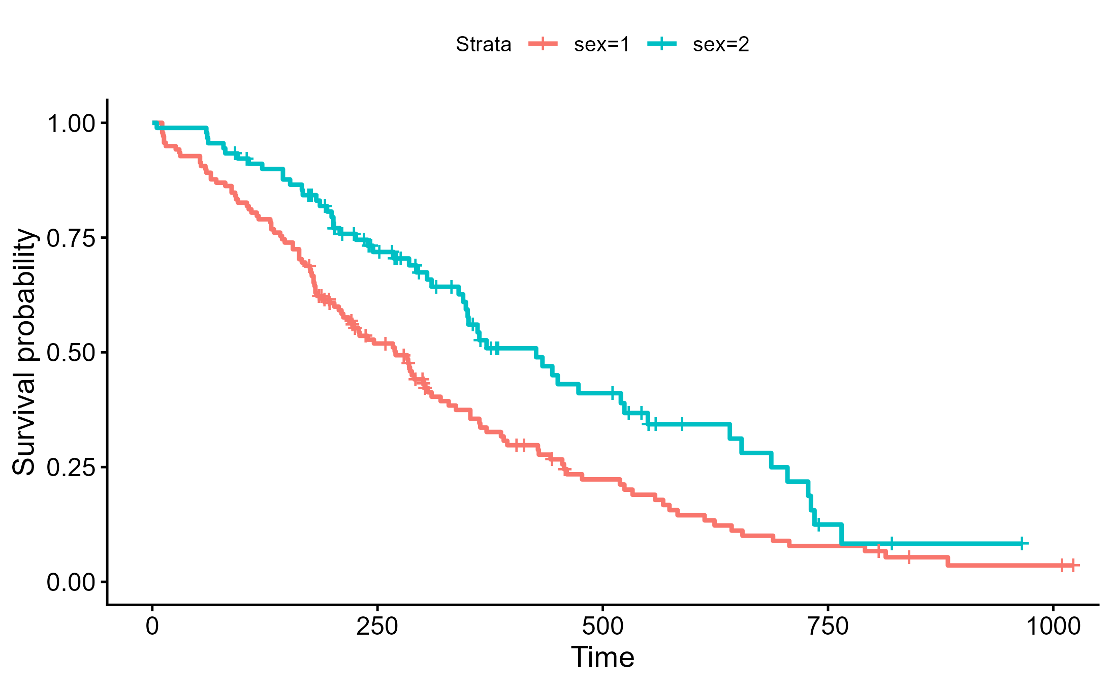
png("./images/KM_detail.png", width = 1000, height = 1000, res = 120)
ggsurvplot(sfit, conf.int=TRUE, pval=TRUE, risk.table=TRUE,
           legend.labs=c("Male", "Female"), legend.title="Sex",
           palette=c("dodgerblue2", "orchid2"),
           title="Kaplan-Meier Curve for Lung Cancer Survival",
           risk.table.height=.15)
dev.off()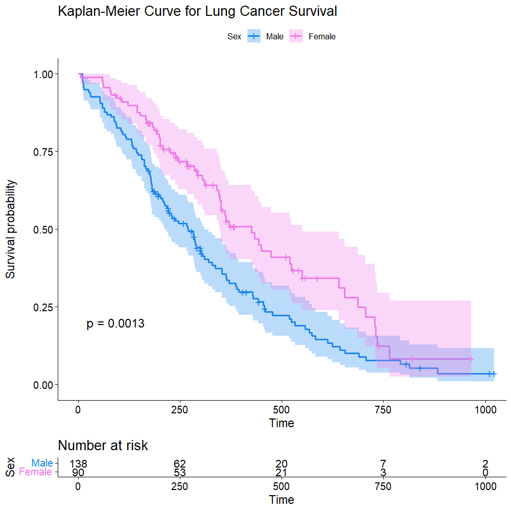
6 Cox回歸
fit <- coxph(Surv(time, status)~sex, data=lung)
fit
Call:
coxph(formula = Surv(time, status) ~ sex, data = lung)
coef exp(coef) se(coef) z p
sex -0.5310 0.5880 0.1672 -3.176 0.00149
Likelihood ratio test=10.63 on 1 df, p=0.001111
n= 228, number of events= 165 summary(fit)
survdiff(Surv(time, status)~sex, data=lung)Call:
coxph(formula = Surv(time, status) ~ sex, data = lung)
n= 228, number of events= 165
coef exp(coef) se(coef) z Pr(>|z|)
sex -0.5310 0.5880 0.1672 -3.176 0.00149 **
---
Signif. codes: 0 ‘***’ 0.001 ‘**’ 0.01 ‘*’ 0.05 ‘.’ 0.1 ‘ ’ 1
exp(coef) exp(-coef) lower .95 upper .95
sex 0.588 1.701 0.4237 0.816
Concordance= 0.579 (se = 0.021 )
Likelihood ratio test= 10.63 on 1 df, p=0.001
Wald test = 10.09 on 1 df, p=0.001
Score (logrank) test = 10.33 on 1 df, p=0.001
Call:
survdiff(formula = Surv(time, status) ~ sex, data = lung)
N Observed Expected (O-E)^2/E (O-E)^2/V
sex=1 138 112 91.6 4.55 10.3
sex=2 90 53 73.4 5.68 10.3
Chisq= 10.3 on 1 degrees of freedom, p= 0.001 fit <- coxph(Surv(time, status)~sex+age+ph.ecog+ph.karno+pat.karno+meal.cal+wt.loss, data=lung)
fitCall:
coxph(formula = Surv(time, status) ~ sex + age + ph.ecog + ph.karno +
pat.karno + meal.cal + wt.loss, data = lung)
coef exp(coef) se(coef) z p
sex -5.509e-01 5.765e-01 2.008e-01 -2.743 0.00609
age 1.065e-02 1.011e+00 1.161e-02 0.917 0.35906
ph.ecog 7.342e-01 2.084e+00 2.233e-01 3.288 0.00101
ph.karno 2.246e-02 1.023e+00 1.124e-02 1.998 0.04574
pat.karno -1.242e-02 9.877e-01 8.054e-03 -1.542 0.12316
meal.cal 3.329e-05 1.000e+00 2.595e-04 0.128 0.89791
wt.loss -1.433e-02 9.858e-01 7.771e-03 -1.844 0.06518
Likelihood ratio test=28.33 on 7 df, p=0.0001918
n= 168, number of events= 121
(因為不存在,60 個觀察量被刪除了)7 KM plot分組
先查看適合切點
mean(lung$age)
ggplot(lung, aes(age)) + geom_histogram(bins=20)
ggsave("./images/histogram.png")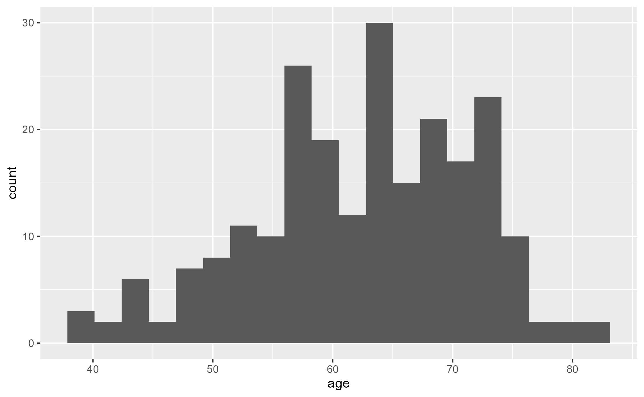
lung <- lung %>%
  dplyr::mutate(agecat=cut(age, breaks=c(0, 62, Inf), labels=c("young", "old")))

head(lung)| inst | time | status | age | sex | ph.ecog | ph.karno | pat.karno | meal.cal | wt.loss | agecat |
|---|---|---|---|---|---|---|---|---|---|---|
| 3 | 306 | 2 | 74 | 1 | 1 | 90 | 100 | 1175 | NA | old |
| 3 | 455 | 2 | 68 | 1 | 0 | 90 | 90 | 1225 | 15 | old |
| 3 | 1010 | 1 | 56 | 1 | 0 | 90 | 90 | NA | 15 | young |
| 5 | 210 | 2 | 57 | 1 | 0 | 90 | 60 | 1150 | 11 | young |
| 1 | 883 | 2 | 60 | 1 | 0 | 100 | 90 | NA | 0 | young |
| 12 | 1022 | 1 | 74 | 1 | 1 | 50 | 80 | 513 | 0 | old |
ggsurvplot(survfit(Surv(time, status)~agecat, data=lung), pval=TRUE)
ggsave("./images/survival_cut.png")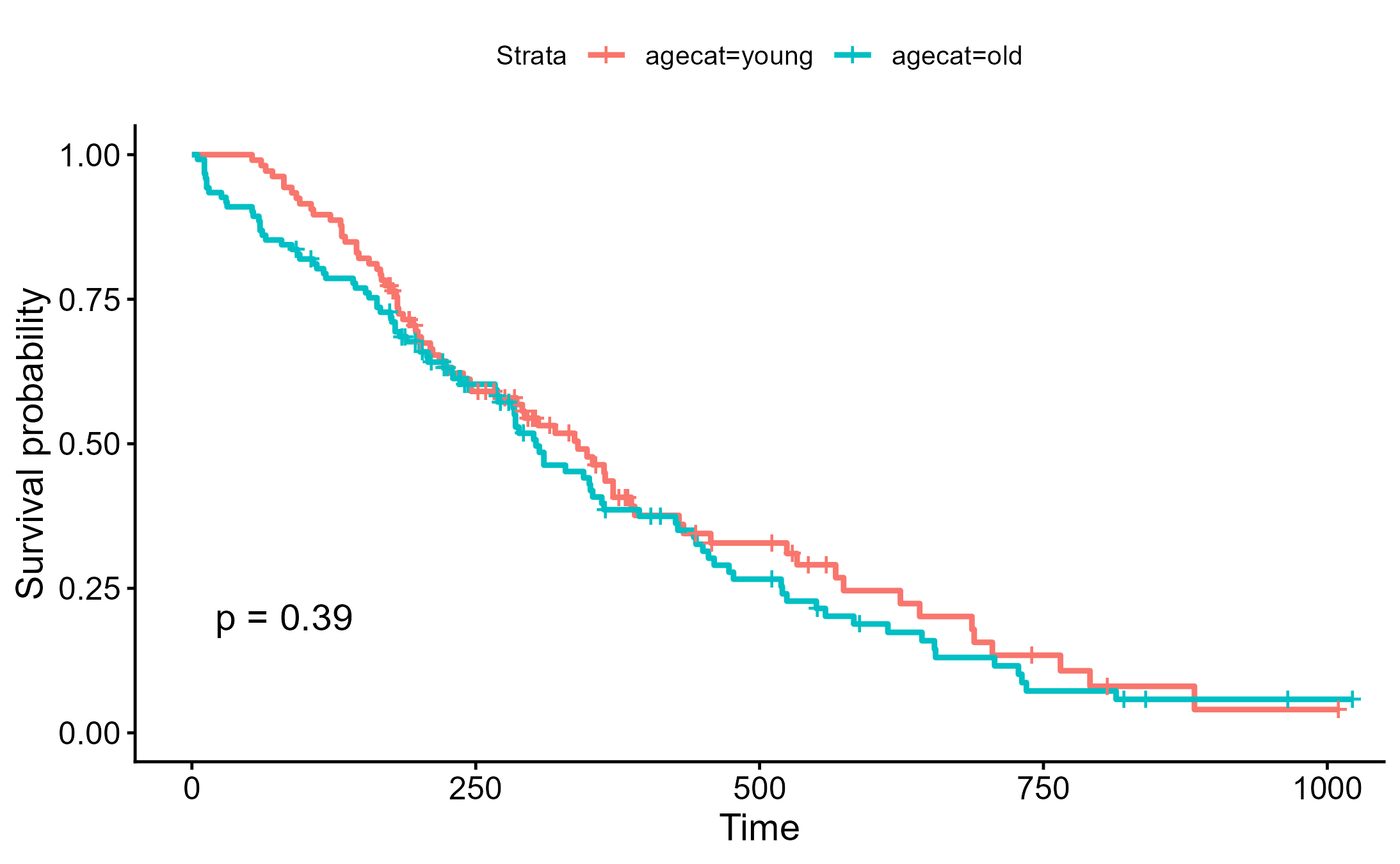
不同切點
lung <- lung %>%
  dplyr::mutate(agecat=cut(age, breaks=c(0, 70, Inf), labels=c("young", "old")))

ggsurvplot(survfit(Surv(time, status)~agecat, data=lung), pval=TRUE)
ggsave("./images/survival_cut2.png")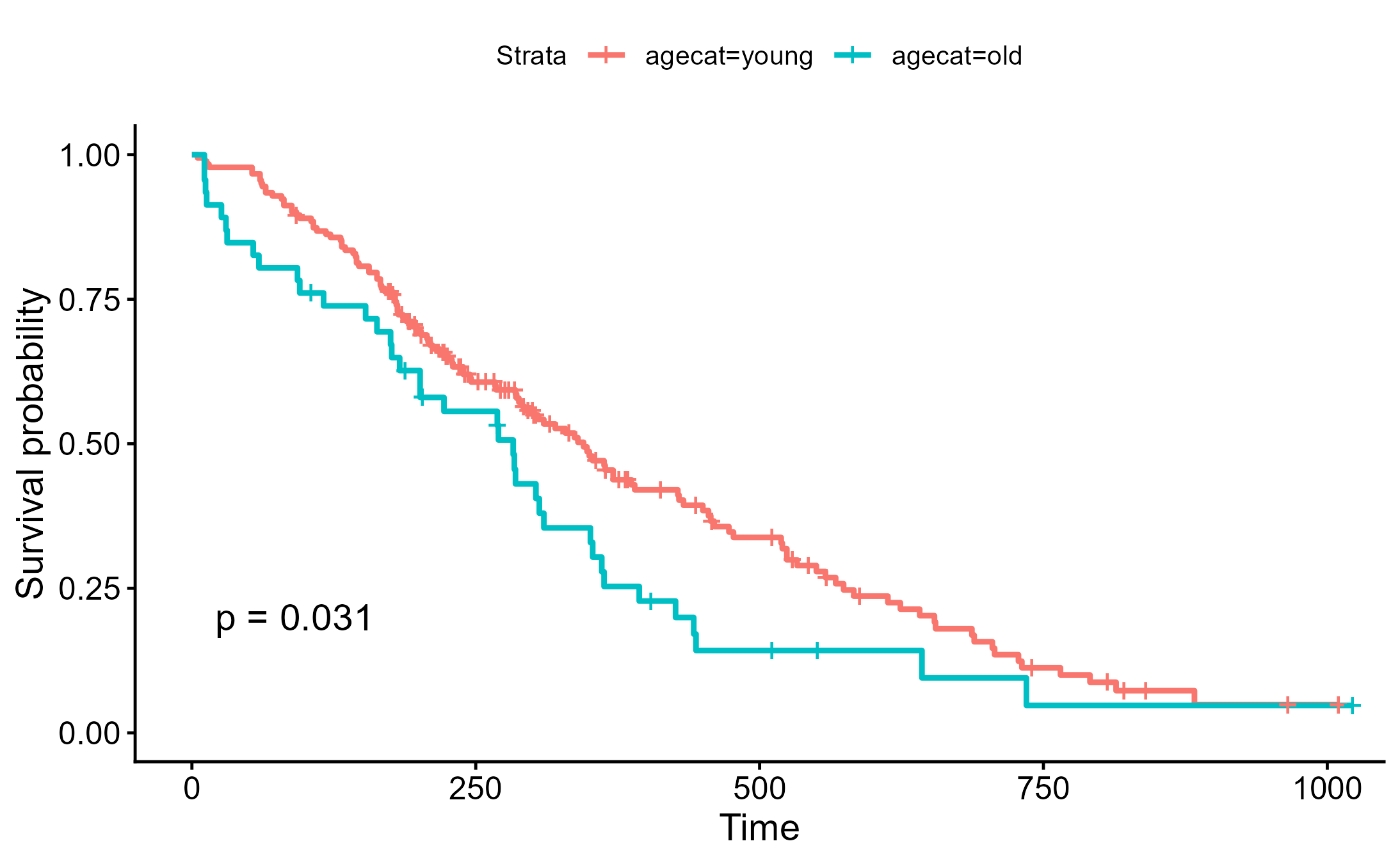
8 ROC
- status
1= censored(未發生事件,截尾)
2= dead(事件發生)
- event
1= event(事件發生)
0= without event(未發生事件)
analysis_df <- lung_df %>%
  dplyr::mutate(event = as.integer(status == 2)) %>%
  dplyr::select(time, event, age, sex, ph.ecog) %>%
  tidyr::drop_na()

cox_fit <- analysis_df %>%
  survival::coxph(Surv(time, event) ~ age + sex + ph.ecog, data = .)

summary(cox_fit)
Call:
survival::coxph(formula = Surv(time, event) ~ age + sex + ph.ecog,
data = .)
n= 227, number of events= 164
coef exp(coef) se(coef) z Pr(>|z|)
age 0.011067 1.011128 0.009267 1.194 0.232416
sex -0.552612 0.575445 0.167739 -3.294 0.000986 ***
ph.ecog 0.463728 1.589991 0.113577 4.083 4.45e-05 ***
---
Signif. codes: 0 ‘***’ 0.001 ‘**’ 0.01 ‘*’ 0.05 ‘.’ 0.1 ‘ ’ 1
exp(coef) exp(-coef) lower .95 upper .95
age 1.0111 0.9890 0.9929 1.0297
sex 0.5754 1.7378 0.4142 0.7994
ph.ecog 1.5900 0.6289 1.2727 1.9864
Concordance= 0.637 (se = 0.025 )
Likelihood ratio test= 30.5 on 3 df, p=1e-06
Wald test = 29.93 on 3 df, p=1e-06
Score (logrank) test = 30.5 on 3 df, p=1e-06risk_score <- predict(cox_fit, type = "lp")
head(risk_score)[1] 0.3692998 -0.1608293 -0.2936304 0.1811648 -0.2493634 0.3692998times_years <- c(0.5, 1, 2)
times_days <- times_years * 365
time_roc_res <- timeROC(
T = analysis_df$time,
delta = analysis_df$event,
marker = risk_score,
cause = 1,
times = times_days,
iid = TRUE
)
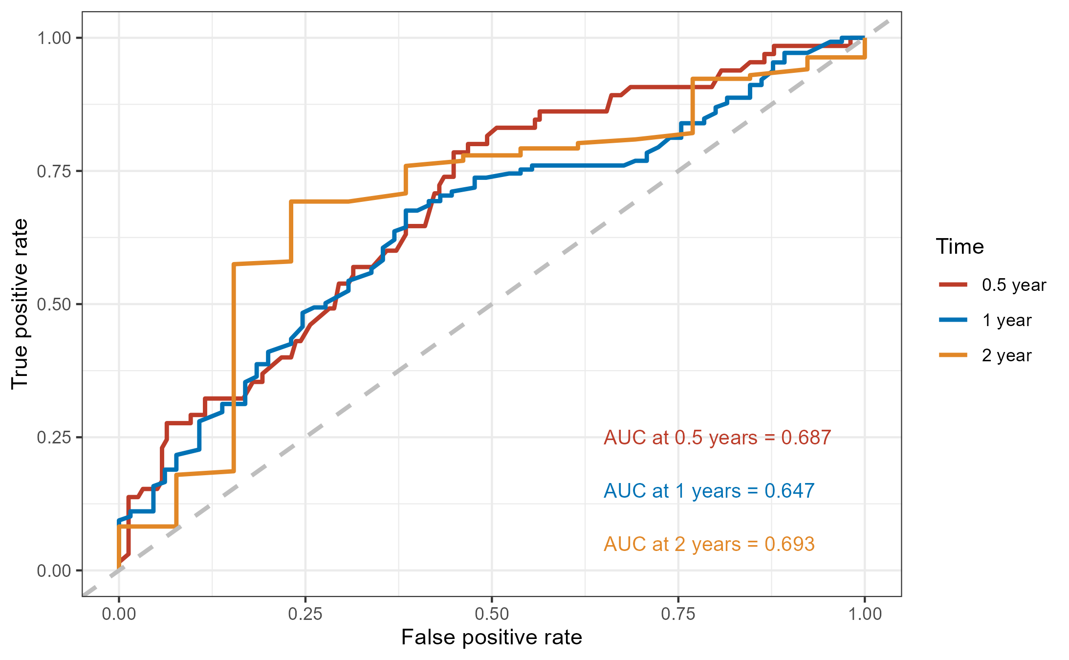
time_roc_res$AUC t=182.5 t=365 t=730
0.6870773 0.6473977 0.6933593 roc_df <- map_dfr(
seq_along(times_years),
function(i) {
tibble(
FPR = time_roc_res$FP[, i],
TPR = time_roc_res$TP[, i],
time = paste0(times_years[i], " year")
)
}
)
head(roc_df)| FPR | TPR | time |
|---|---|---|
| 0.0000000 | 0.0000000 | 0.5 year |
| 0.0000000 | 0.01540802 | 0.5 year |
| 0.01282051 | 0.03066037 | 0.5 year |
| 0.01282051 | 0.07649409 | 0.5 year |
| 0.01282051 | 0.09174645 | 0.5 year |
| 0.01282051 | 0.13765918 | 0.5 year |
plot_time_roc <- function(roc_df, auc, times_years,
                          colors = c("#BC3C29FF", "#0072B5FF", "#E18727FF")) {

  auc_labels <- paste0(
    "AUC at ", times_years, " years = ",
    sprintf("%.3f", auc)
  )

  ggplot(roc_df, aes(x = FPR, y = TPR, color = time)) +
    geom_line(size = 1) +
    geom_abline(
      slope = 1, intercept = 0,
      color = "grey", linetype = "dashed", size = 1
    ) +
    scale_color_manual(values = colors) +
    theme_bw() +
    labs(
      x = "False positive rate",
      y = "True positive rate",
      color = "Time"
    ) +
    annotate(
      "text",
      x = 0.65,
      y = seq(0.25, 0.25 - 0.1 * (length(auc_labels) - 1), by = -0.1),
      label = auc_labels,
      color = colors,
      size = 3.5,
      hjust = 0
    )
}plot_time_roc(
roc_df = roc_df,
auc = time_roc_res$AUC,
times_years = times_years
)
ggsave("./images/ROC_curve.png")