library("tximport")
library("readr")
library("tximportData")

# get sample information
dir <- system.file("extdata", package="tximportData")
sample_info <- read.table(file.path(dir,"samples.txt"), header=TRUE)
rownames(sample_info) <- sample_info$run

# mimic no-replicates
sample_info$condition <- factor(rep(c("A","B","C","D","E","F")))
head(sample_info)rnaseq-no-replicates-edger
1 匯入樣本
本 workflow 使用 tximportData 套件提供的資料進行示範
Important
進行差異表達(DE)分析前,需具備完整的樣本與定量資訊,包括:
- 樣本的 metadata(分組、條件與樣本識別碼)
- 轉錄本定量工具(如 kallisto)輸出的 count 資料
- 將轉錄本彙整至基因層級所需的 tx2gene 對照表
1.1 metadata
Important
樣本的 metadata 在分析流程中具有關鍵作用,用於記錄每個樣本所對應的實驗條件、分組資訊與相關註解。建議以結構化格式(如 csv 或 txt 檔案)進行整理與匯入,以利後續分析與流程自動化。
Note
為了模擬沒有生物重複的樣本,我們設定 condition 是 A 到 F 不同狀況
          pop center                assay    sample experiment       run condition
ERR188297 TSI  UNIGE NA20503.1.M_111124_5 ERS185497  ERX163094 ERR188297         A
ERR188088 TSI  UNIGE NA20504.1.M_111124_7 ERS185242  ERX162972 ERR188088         B
ERR188329 TSI  UNIGE NA20505.1.M_111124_6 ERS185048  ERX163009 ERR188329         C
ERR188288 TSI  UNIGE NA20507.1.M_111124_7 ERS185412  ERX163158 ERR188288         D
ERR188021 TSI  UNIGE NA20508.1.M_111124_2 ERS185362  ERX163159 ERR188021         E
ERR188356 TSI  UNIGE NA20514.1.M_111124_4 ERS185217  ERX163062 ERR188356         F
1.2 tx2gene mapping
Important
由於 RNA-seq 定量工具(如 kallisto)輸出的計數資料通常位於轉錄本(transcript)層級,而後續差異表達分析多以基因(gene)層級進行,因此需要透過 tx2gene 對照表,將轉錄本層級的定量結果彙總至基因層級。
此類轉錄本與基因之間的對應關係可由公開註解資料取得,例如可自 GENCODE(Ensembl)或 NCBI RefSeq 等來源下載對應物種的 GTF 註解檔,並由其中擷取 transcript ID 與 gene ID 的對照資訊,以建立 tx2gene 映射表。
外部連結: ensembl release-113 gtf
Note
本範例資料使用 kallisto 進行定量,其輸出的轉錄本 ID 不包含版本號後綴(如 .1, .2)。為確保 tx2gene 對照正確,需將對照表中轉錄本與基因 ID 的版本號後綴一併移除。
# 同樣使用 `tximportData` 提供的 tx2gene table
tx2gene <- read_csv(file.path(dir, "tx2gene.gencode.v27.csv"))

# 移除版本號後綴
tx2gene$TXNAME <- sub("\\..*$", "", tx2gene$TXNAME)
tx2gene$GENEID <- sub("\\..*$", "", tx2gene$GENEID)
head(tx2gene)
Rows: 200401 Columns: 2
── Column specification ────────────────────────────────────────────────────────────────────────────────────────────────────────────────────
Delimiter: ","
chr (2): TXNAME, GENEID
ℹ Use `spec()` to retrieve the full column specification for this data.
ℹ Specify the column types or set `show_col_types = FALSE` to quiet this message.
# A tibble: 6 × 2
TXNAME GENEID
<chr> <chr>
1 ENST00000456328 ENSG00000223972
2 ENST00000450305 ENSG00000223972
3 ENST00000473358 ENSG00000243485
4 ENST00000469289 ENSG00000243485
5 ENST00000607096 ENSG00000284332
6 ENST00000606857 ENSG000002680201.3 count matrix
# 列出所有樣本對應的 kallisto 定量檔案路徑(abundance.h5)
# 並將樣本名稱指定為 list 的 key,以確保匯入後的欄位名稱
# 能正確對應到 metadata 中的樣本順序與識別碼
files <- file.path(dir,"kallisto", samples$run, "abundance.h5")
names(files) <- sample_info$run
files
ERR188297
"C:/Users/benson_lee/AppData/Local/R/win-library/4.4/tximportData/extdata/kallisto/ERR188297/abundance.h5"
ERR188088
"C:/Users/benson_lee/AppData/Local/R/win-library/4.4/tximportData/extdata/kallisto/ERR188088/abundance.h5"
ERR188329
"C:/Users/benson_lee/AppData/Local/R/win-library/4.4/tximportData/extdata/kallisto/ERR188329/abundance.h5"
ERR188288
"C:/Users/benson_lee/AppData/Local/R/win-library/4.4/tximportData/extdata/kallisto/ERR188288/abundance.h5"
ERR188021
"C:/Users/benson_lee/AppData/Local/R/win-library/4.4/tximportData/extdata/kallisto/ERR188021/abundance.h5"
ERR188356
"C:/Users/benson_lee/AppData/Local/R/win-library/4.4/tximportData/extdata/kallisto/ERR188356/abundance.h5"
Note
根據上游分析的工具,設定 tximport 函數的 type 參數,常見可用的有 salmon, kallisto 與 rsem 等等,若要詳細瞭解可以在 R 中輸入 ?tximport 看詳細資料,也可以參考tximport套件官方說明了解該函數的用法
# 使用 tximport 將轉錄本層級的定量結果匯入,
# 並透過 tx2gene 對照表彙整為基因層級的 count matrix
txi.kallisto <- tximport::tximport(
  files = files,
  type = "kallisto",
  tx2gene = tx2gene,
  txOut = FALSE,
  ignoreTxVersion = TRUE
)
1 2 3 4 5 6
removing duplicated transcript rows from tx2gene
summarizing abundance
summarizing counts
summarizing length1.4 建立 DGEList 物件
Important
此步驟僅是將基因層級的 count matrix 與樣本 metadata
封裝成 edgeR 可辨識的 DGEList 物件,尚未進行任何正規化或差異表達分析。
後續仍需依序進行 library size 校正、離群基因過濾、模型建立與統計檢定。
library(edgeR)

dge <- edgeR::DGEList(
  counts = txi.kallisto$counts,
  samples = sample_info
)

dge
class(dge)
An object of class "DGEList"
$counts
ERR188297 ERR188088 ERR188329 ERR188288 ERR188021 ERR188356
ENSG00000000003 2.597454 2.0000 27.15883 8.406228 5.064623 5.741246
ENSG00000000005 0.000000 0.0000 0.00000 0.000000 0.000000 0.000000
ENSG00000000419 1057.000000 1338.0000 1453.00000 1289.000000 921.000000 1332.000000
ENSG00000000457 462.528935 495.4176 564.18466 385.988581 532.848389 543.533790
ENSG00000000460 630.398169 418.5461 1166.26652 611.513416 915.493338 636.256168
58238 more rows ...
$samples
group lib.size norm.factors pop center assay sample experiment run condition
ERR188297 1 22844138 1 TSI UNIGE NA20503.1.M_111124_5 ERS185497 ERX163094 ERR188297 A
ERR188088 1 23742623 1 TSI UNIGE NA20504.1.M_111124_7 ERS185242 ERX162972 ERR188088 B
ERR188329 1 34513836 1 TSI UNIGE NA20505.1.M_111124_6 ERS185048 ERX163009 ERR188329 C
ERR188288 1 23867902 1 TSI UNIGE NA20507.1.M_111124_7 ERS185412 ERX163158 ERR188288 D
ERR188021 1 28702608 1 TSI UNIGE NA20508.1.M_111124_2 ERS185362 ERX163159 ERR188021 E
ERR188356 1 22615555 1 TSI UNIGE NA20514.1.M_111124_4 ERS185217 ERX163062 ERR188356 F
[1] "DGEList"
attr(,"package")
[1] "edgeR"
Note
以上是讀取資料的部分,接下來是針對 dge 物件進行各種前處理操作,包含過濾低表現量的基因以及TMM標準化
2 前處理
2.1 過濾低表現基因(篩選)
cpm_mat <- edgeR::cpm(dge)
keep <- rowSums(cpm_mat >= 1) >= (ncol(dge) / 2)    # 篩選:至少一半樣本CPM >= 1
dge_filt <- dge[keep, , keep.lib.sizes = FALSE]
2.2 過濾低表現基因(繪圖)
library(RColorBrewer)

lcpm_raw <- cpm(dge, log = TRUE)
cpm_cutoff <- log2(1 + 1e-6)
nsamples <- ncol(dge)
col <- brewer.pal(nsamples, "Paired")

png("./images/filter_cpm_density.png", width = 2000, height = 1000, res = 200)
par(mfrow = c(1, 2), mar = c(5, 5, 4, 2))

# ----------------------------
# A. Before filtering
# ----------------------------
plot(density(lcpm_raw[,1]), col = col[1], lwd = 2,
     ylim = c(0, 0.3), main = "", xlab = "log2-CPM")
title(main = "A. Before CPM filtering")
abline(v = cpm_cutoff, lty = 3)

for (i in 2:nsamples) {
  den <- density(lcpm_raw[,i])
  lines(den$x, den$y, col = col[i], lwd = 2)
}

legend("topright", colnames(dge), text.col = col, bty = "n")

# ----------------------------
# B. After filtering
# ----------------------------
lcpm_filt <- cpm(dge_filt, log = TRUE)

plot(density(lcpm_filt[,1]), col = col[1], lwd = 2,
     ylim = c(0, 0.3), main = "", xlab = "log2-CPM")
title(main = "B. After CPM filtering")
abline(v = cpm_cutoff, lty = 3)

for (i in 2:ncol(dge_filt)) {
  den <- density(lcpm_filt[,i])
  lines(den$x, den$y, col = col[i], lwd = 2)
}

legend("topright", colnames(dge_filt), text.col = col, bty = "n")

dev.off()
par(mfrow = c(1,1))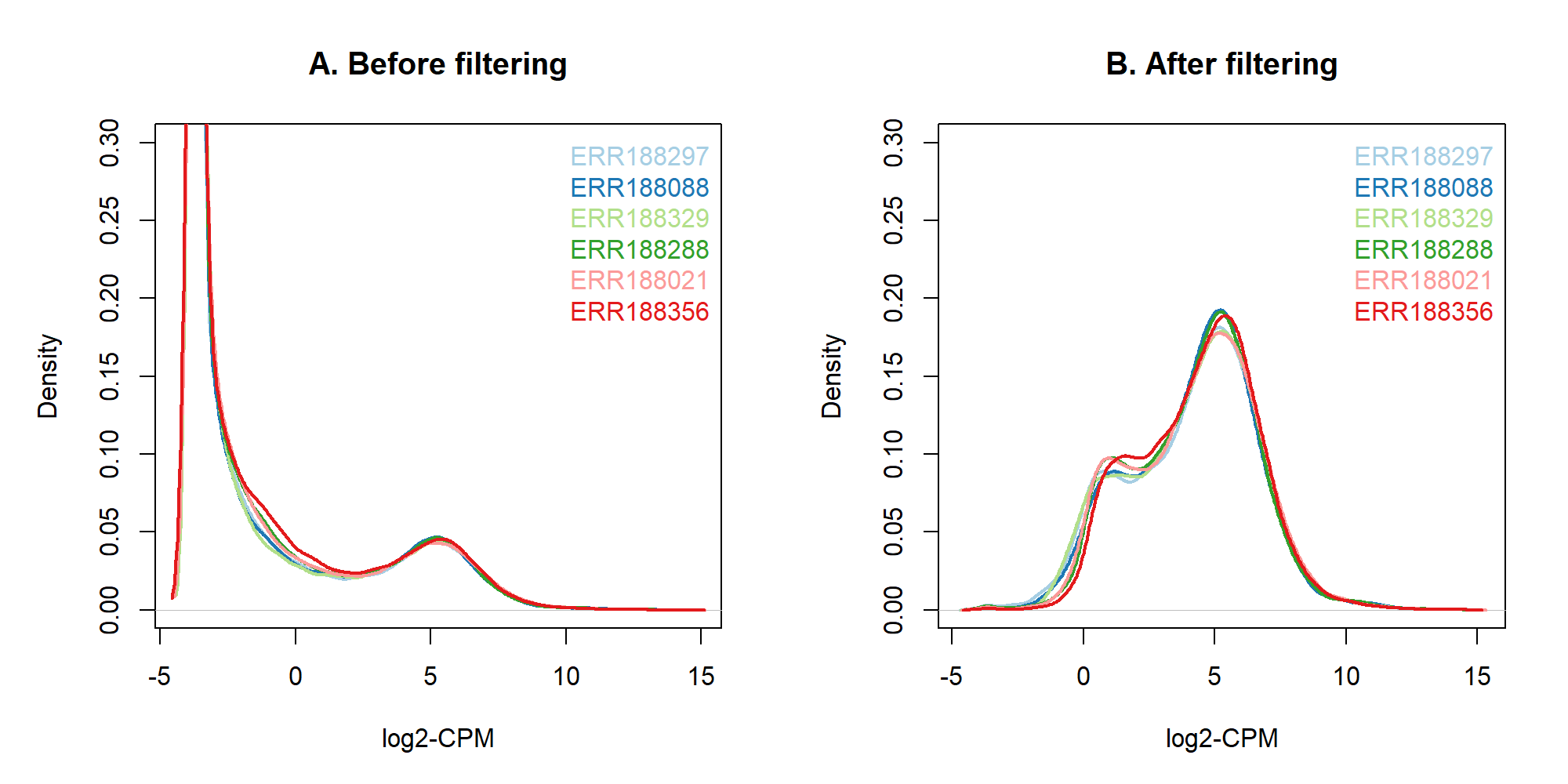
2.3 過濾低表現基因(自訂繪圖函式)
plot_cpm_density() 函式版本(點擊展開)
plot_cpm_density <- function(
  dge_raw,
  dge_filt,
  outfile = "./filter_cpm_density.png",
  palette = "Paired",
  ylim = c(0, 0.3),
  width = 2000,
  height = 1000,
  res = 200,
  prior_count = 2
) {
  # ----------------------------
  # Input checks
  # ----------------------------
  if (!inherits(dge_raw, "DGEList"))
    stop("`dge_raw` must be an edgeR DGEList object")

  if (!inherits(dge_filt, "DGEList"))
    stop("`dge_filt` must be an edgeR DGEList object")

  if (!requireNamespace("edgeR", quietly = TRUE))
    stop("Package 'edgeR' is required")

  if (!requireNamespace("RColorBrewer", quietly = TRUE))
    stop("Package 'RColorBrewer' is required")

  # ----------------------------
  # log-CPM calculation
  # ----------------------------
  lcpm_raw  <- edgeR::cpm(dge_raw,  log = TRUE, prior.count = prior_count)
  lcpm_filt <- edgeR::cpm(dge_filt, log = TRUE, prior.count = prior_count)

  nsamples <- ncol(dge_raw)

  # 檢查 palette 是否支援樣本數
  max_cols <- RColorBrewer::brewer.pal.info[palette, "maxcolors"]
  if (nsamples > max_cols) {
    stop(
      sprintf(
        "Palette '%s' supports up to %d colors, but nsamples = %d.",
        palette, max_cols, nsamples
      )
    )
  }
  cols <- RColorBrewer::brewer.pal(nsamples, palette)

  # ----------------------------
  # Plot
  # ----------------------------
  png(outfile, width = width, height = height, res = res)
  op <- par(mfrow = c(1, 2), mar = c(5, 5, 4, 2))
  on.exit({ par(op); dev.off() }, add = TRUE)

  ## A. Before filtering
  plot(
    density(lcpm_raw[, 1]),
    col = cols[1], lwd = 2,
    ylim = ylim,
    xlab = "log2-CPM",
    main = "A. Before filtering"
  )
  for (i in 2:nsamples) {
    lines(density(lcpm_raw[, i]), col = cols[i], lwd = 2)
  }
  legend("topright", colnames(dge_raw), text.col = cols, bty = "n")

  ## B. After filtering
  plot(
    density(lcpm_filt[, 1]),
    col = cols[1], lwd = 2,
    ylim = ylim,
    xlab = "log2-CPM",
    main = "B. After filtering"
  )
  for (i in 2:ncol(dge_filt)) {
    lines(density(lcpm_filt[, i]), col = cols[i], lwd = 2)
  }
  legend("topright", colnames(dge_filt), text.col = cols, bty = "n")

  invisible(outfile)
}plot_cpm_density(
dge_raw = dge,
dge_filt = dge_filt,
outfile = "./images/filter_cpm_density.png")2.4 TMM
dge_norm <- calcNormFactors(dge_filt, method = c("TMM"))
dge_norm$samples
group lib.size norm.factors pop center assay sample experiment run condition
ERR188297 1 22774970 0.9826883 TSI UNIGE NA20503.1.M_111124_5 ERS185497 ERX163094 ERR188297 A
ERR188088 1 23663007 0.9772987 TSI UNIGE NA20504.1.M_111124_7 ERS185242 ERX162972 ERR188088 B
ERR188329 1 34399139 0.9755415 TSI UNIGE NA20505.1.M_111124_6 ERS185048 ERX163009 ERR188329 C
ERR188288 1 23746536 0.9969002 TSI UNIGE NA20507.1.M_111124_7 ERS185412 ERX163158 ERR188288 D
ERR188021 1 28594120 1.0159830 TSI UNIGE NA20508.1.M_111124_2 ERS185362 ERX163159 ERR188021 E
ERR188356 1 22469952 1.0538359 TSI UNIGE NA20514.1.M_111124_4 ERS185217 ERX163062 ERR188356 F2.5 TMM(繪圖)
library(RColorBrewer)

nsamples <- ncol(dge_filt)
col <- brewer.pal(nsamples, "Paired")
dge_filt$samples$norm.factors <- 1

png("./images/tmm_boxplot_realdata.png", width=2000, height=1000, res=200)
par(mfrow=c(1,2))

boxplot(cpm(dge_filt, log=TRUE), las=2, col=col, outline=FALSE,
        main="A. Before TMM", ylab="log2-CPM")

boxplot(cpm(dge_norm, log=TRUE), las=2, col=col, outline=FALSE,
        main="B. After TMM", ylab="log2-CPM")

dev.off()
par(mfrow=c(1,1))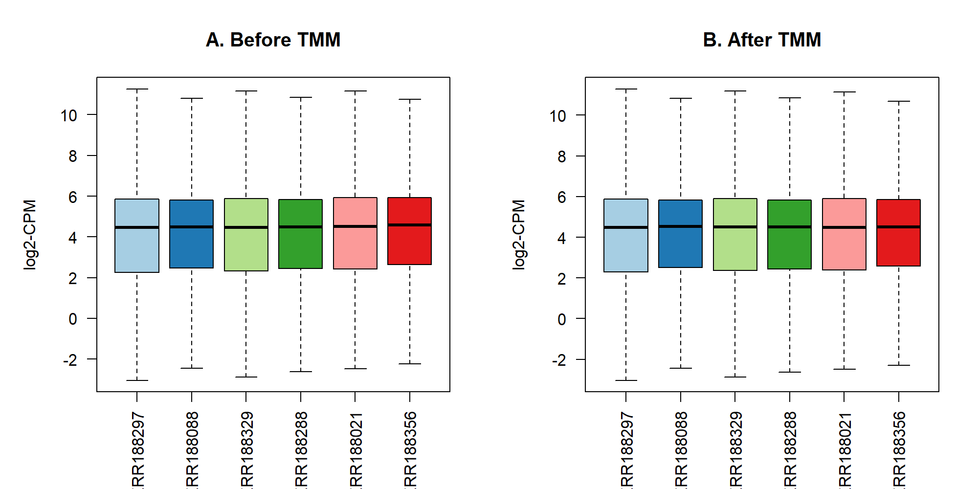
2.6 TMM(自訂繪圖函式)
plot_tmm_boxplot() 函式版本(點擊展開)
plot_tmm_boxplot <- function(
  dge,
  outfile = "./tmm_boxplot_realdata.png",
  palette = "Paired",
  width = 2000,
  height = 1000,
  res = 200
) {
  # ----------------------------
  # Input checks
  # ----------------------------
  if (!inherits(dge, "DGEList"))
    stop("`dge` must be an edgeR DGEList object")

  if (!requireNamespace("edgeR", quietly = TRUE))
    stop("Package 'edgeR' is required")

  if (!requireNamespace("RColorBrewer", quietly = TRUE))
    stop("Package 'RColorBrewer' is required")

  nsamples <- ncol(dge)

  max_cols <- RColorBrewer::brewer.pal.info[palette, "maxcolors"]
  if (nsamples > max_cols) {
    stop(
      sprintf(
        "Palette '%s' supports up to %d colors, but nsamples = %d.",
        palette, max_cols, nsamples
      )
    )
  }
  cols <- RColorBrewer::brewer.pal(nsamples, palette)

  # ----------------------------
  # Before TMM: force norm.factors = 1
  # ----------------------------
  dge_before <- dge
  dge_before$samples$norm.factors <- 1

  # ----------------------------
  # After TMM
  # ----------------------------
  dge_after <- edgeR::calcNormFactors(dge_before)

  # ----------------------------
  # Plot
  # ----------------------------
  png(outfile, width = width, height = height, res = res)
  op <- par(mfrow = c(1, 2), mar = c(5, 5, 4, 2))
  on.exit({ par(op); dev.off() }, add = TRUE)

  ## A. Before TMM
  boxplot(
    edgeR::cpm(dge_before, log = TRUE),
    las = 2,
    col = cols,
    outline = FALSE,
    main = "A. Before TMM",
    ylab = "log2-CPM"
  )

  ## B. After TMM
  boxplot(
    edgeR::cpm(dge_after, log = TRUE),
    las = 2,
    col = cols,
    outline = FALSE,
    main = "B. After TMM",
    ylab = "log2-CPM"
  )

  invisible(list(
    dge_before = dge_before,
    dge_after  = dge_after,
    outfile    = outfile
  ))
}plot_tmm_boxplot(dge_filt, outfile = "./images/tmm_boxplot_realdata.png")3 DE分析
3.1 手動設定 dispersion
Important
在缺乏生物重複(no biological replicates)的情況下,edgeR 無法從資料中可靠地估計離散度(dispersion)。因此,此處手動指定 common dispersion(例如 0.05),僅作為示範與流程展示用途。
實際研究分析中,建議至少包含生物重複,並透過 estimateDisp() 由資料本身估計 dispersion,以確保統計推論的可靠性。
# Common dispersion manually set to 0.05 because no biological replicates
dge_norm$common.dispersion <- 0.05
3.2 設定 design
design <- model.matrix(~0 + condition, data = dge_norm$samples)
colnames(design) <- levels(dge_norm$samples$condition)
design
A B C D E F
ERR188297 1 0 0 0 0 0
ERR188088 0 1 0 0 0 0
ERR188329 0 0 1 0 0 0
ERR188288 0 0 0 1 0 0
ERR188021 0 0 0 0 1 0
ERR188356 0 0 0 0 0 1
attr(,"assign")
[1] 1 1 1 1 1 1
attr(,"contrasts")
attr(,"contrasts")$condition
[1] "contr.treatment"3.3 (手動)設定 contrast
對照放後面
contrast_matrix <- makeContrasts(
   BvsA = B - A,
   CvsA = C - A,
   levels = colnames(design))
contrast_matrix
Contrasts
Levels BvsA CvsA
A -1 -1
B 1 0
C 0 1
D 0 0
E 0 0
F 0 03.4 (進階)匯入 contrast
comparisons.csv:
Treatment,Control
B,A
C,A
D,A
E,A
F,A
B,C
comparisons <- read.csv("data/comparisons.csv", stringsAsFactors = FALSE)
comparisons Treatment Control
1 B A
2 C A
3 D A
4 E A
5 F A
6 B Cmake_contrast_matrix <- function(comparisons, design) {
levs <- colnames(design)
n_comp <- nrow(comparisons)
contrast_matrix <- matrix(
0,
nrow = length(levs),
ncol = n_comp,
dimnames = list(
levs,
paste0(comparisons$Treatment, "vs", comparisons$Control)
)
)
for (i in seq_len(n_comp)) {
contrast_matrix[comparisons$Treatment[i], i] <- 1
contrast_matrix[comparisons$Control[i], i] <- -1
}
contrast_matrix
}contrast_matrix <- make_contrast_matrix(comparisons, design)
contrast_matrix BvsA CvsA DvsA EvsA FvsA BvsC
A -1 -1 -1 -1 -1 0
B 1 0 0 0 0 1
C 0 1 0 0 0 -1
D 0 0 1 0 0 0
E 0 0 0 1 0 0
F 0 0 0 0 1 04 GLM 模型
4.1 GLM fitting
fit <- glmFit(dge_norm, design)4.2 Likelihood ratio tests
# 以下兩個指令等價,但上面更直觀
lrt <- glmLRT(fit, contrast = contrast_matrix[, "BvsA"])
lrt <- glmLRT(fit, contrast = c(-1, 1, 0, 0, 0, 0))

# 使用 `topTags` 索引結果
topTags(lrt)
Coefficient: 1*A -1*B
logFC logCPM LR PValue FDR
ENSG00000211644 8.602423 7.706599 176.7697 2.459000e-40 3.432519e-36
ENSG00000244398 -14.290756 5.707485 172.4603 2.147016e-39 1.498510e-35
ENSG00000211947 7.789757 7.727715 158.0047 3.087496e-36 1.436612e-32
ENSG00000240342 7.174882 7.069052 135.6556 2.373213e-31 8.281920e-28
ENSG00000211659 -7.972426 5.947324 131.1426 2.304456e-30 6.433581e-27
ENSG00000211966 -6.821394 5.490954 126.0942 2.932350e-29 6.822113e-26
ENSG00000090530 7.434324 3.640713 116.7308 3.288038e-27 6.556818e-24
ENSG00000184368 -7.122196 3.951757 116.1274 4.457148e-27 7.777166e-24
ENSG00000211648 6.814211 5.354604 114.9717 7.982812e-27 1.238134e-23
ENSG00000137731 -6.632437 4.777895 112.6390 2.588623e-26 3.613459e-23lrt_results <- lapply(colnames(contrast_matrix), function(cn) {
glmLRT(fit, contrast = contrast_matrix[, cn])
})
names(lrt_results) <- colnames(contrast_matrix)
topTags(lrt_results[["BvsA"]])Coefficient: -1*A 1*B
logFC logCPM LR PValue FDR
ENSG00000211644 -8.602423 7.706599 176.7697 2.459000e-40 3.432519e-36
ENSG00000244398 14.290756 5.707485 172.4603 2.147016e-39 1.498510e-35
ENSG00000211947 -7.789757 7.727715 158.0047 3.087496e-36 1.436612e-32
ENSG00000240342 -7.174882 7.069052 135.6556 2.373213e-31 8.281920e-28
ENSG00000211659 7.972426 5.947324 131.1426 2.304456e-30 6.433581e-27
ENSG00000211966 6.821394 5.490954 126.0942 2.932350e-29 6.822113e-26
ENSG00000090530 -7.434324 3.640713 116.7308 3.288038e-27 6.556818e-24
ENSG00000184368 7.122196 3.951757 116.1274 4.457148e-27 7.777166e-24
ENSG00000211648 -6.814211 5.354604 114.9717 7.982812e-27 1.238134e-23
ENSG00000137731 6.632437 4.777895 112.6390 2.588623e-26 3.613459e-23