library("tximport")
library("readr")
library("tximportData")
dir <- system.file("extdata", package="tximportData")
samples <- read.table(file.path(dir,"samples.txt"), header=TRUE)
samples$condition <- factor(rep(c("A","B"),each=3))
rownames(samples) <- samples$run
samples[,c("pop","center","run","condition")]RNA-seq deseq2 workflow
TipReference
Love, M.I., Huber, W., Anders, S. (2014) Moderated estimation of fold change and dispersion for RNA-seq data with DESeq2. Genome Biology, 15:550. 10.1186/s13059-014-0550-8
Important
請使用 un-normalized counts 進行分析! DESeq2 模型內部會對 library size 進行校正,因此不應使用經過 transformed 或 normalized 的值作為輸入! 且 DESeq2 必須要有重複樣本才能分析!
1 資料匯入
1.1 (方案一) 使用 tximport
首先需要樣本的 metadata,紀錄樣本的資訊包含 sample name, batch, condition 以及其他重要資訊
          pop center       run condition
ERR188297 TSI  UNIGE ERR188297         A
ERR188088 TSI  UNIGE ERR188088         A
ERR188329 TSI  UNIGE ERR188329         A
ERR188288 TSI  UNIGE ERR188288         B
ERR188021 TSI  UNIGE ERR188021         B
ERR188356 TSI  UNIGE ERR188356         B
接著透過以下方式列出檔案位置,並創建 named-list,key 是樣本名稱,value 是檔案位置
files <- file.path(dir,"salmon", samples$run, "quant.sf.gz")
names(files) <- samples$run
files
ERR188297
"C:/Users/benson_lee/AppData/Local/R/win-library/4.4/tximportData/extdata/salmon/ERR188297/quant.sf.gz"
ERR188088
"C:/Users/benson_lee/AppData/Local/R/win-library/4.4/tximportData/extdata/salmon/ERR188088/quant.sf.gz"
ERR188329
"C:/Users/benson_lee/AppData/Local/R/win-library/4.4/tximportData/extdata/salmon/ERR188329/quant.sf.gz"
ERR188288
"C:/Users/benson_lee/AppData/Local/R/win-library/4.4/tximportData/extdata/salmon/ERR188288/quant.sf.gz"
ERR188021
"C:/Users/benson_lee/AppData/Local/R/win-library/4.4/tximportData/extdata/salmon/ERR188021/quant.sf.gz"
ERR188356
"C:/Users/benson_lee/AppData/Local/R/win-library/4.4/tximportData/extdata/salmon/ERR188356/quant.sf.gz" 準備 tx2gene 對照表
另外由於原始資訊是 ENST transcript 為編號,後續若要合併到基因層級需要對照表 tx2gene。
tx2gene <- read_csv(file.path(dir, "tx2gene.gencode.v27.csv"))
head(tx2gene)
TXNAME GENEID
<chr> <chr>
1 ENST00000456328.2 ENSG00000223972.5
2 ENST00000450305.2 ENSG00000223972.5
3 ENST00000473358.1 ENSG00000243485.5
4 ENST00000469289.1 ENSG00000243485.5
5 ENST00000607096.1 ENSG00000284332.1
6 ENST00000606857.1 ENSG00000268020.3將 files 的檔案匯入,給予 tx2gene 會將 ENST 的 script-id 轉成 gene level的 ENSG,後續用基因層級分析
txi <- tximport(files, type="salmon", tx2gene=tx2gene)reading in files with read_tsv
1 2 3 4 5 6
summarizing abundance
summarizing counts
summarizing length建立 DESeqDataSet 物件
library("DESeq2")
dds_1 <- DESeqDataSetFromTximport(txi,
                                  colData = samples,
                                  design = ~ condition)
using counts and average transcript lengths from tximport1.2 (方案二) 使用 tximeta
Note
Tximeta 是 tximport 的功能擴充版,可以自動添加 metadata
創建 coldata
coldata <- samples
coldata$files <- files
coldata$names <- coldata$run

head(coldata)
pop center assay sample experiment run condition
ERR188297 TSI UNIGE NA20503.1.M_111124_5 ERS185497 ERX163094 ERR188297 A
ERR188088 TSI UNIGE NA20504.1.M_111124_7 ERS185242 ERX162972 ERR188088 A
ERR188329 TSI UNIGE NA20505.1.M_111124_6 ERS185048 ERX163009 ERR188329 A
ERR188288 TSI UNIGE NA20507.1.M_111124_7 ERS185412 ERX163158 ERR188288 B
ERR188021 TSI UNIGE NA20508.1.M_111124_2 ERS185362 ERX163159 ERR188021 B
ERR188356 TSI UNIGE NA20514.1.M_111124_4 ERS185217 ERX163062 ERR188356 B
files names
ERR188297 C:/Users/benson_lee/AppData/Local/R/win-library/4.4/tximportData/extdata/salmon/ERR188297/quant.sf.gz ERR188297
ERR188088 C:/Users/benson_lee/AppData/Local/R/win-library/4.4/tximportData/extdata/salmon/ERR188088/quant.sf.gz ERR188088
ERR188329 C:/Users/benson_lee/AppData/Local/R/win-library/4.4/tximportData/extdata/salmon/ERR188329/quant.sf.gz ERR188329
ERR188288 C:/Users/benson_lee/AppData/Local/R/win-library/4.4/tximportData/extdata/salmon/ERR188288/quant.sf.gz ERR188288
ERR188021 C:/Users/benson_lee/AppData/Local/R/win-library/4.4/tximportData/extdata/salmon/ERR188021/quant.sf.gz ERR188021
ERR188356 C:/Users/benson_lee/AppData/Local/R/win-library/4.4/tximportData/extdata/salmon/ERR188356/quant.sf.gz ERR188356讀檔匯入,此步驟不需提供 tx2gene,因為 tximeta 本身會自動添加註釋
library("tximeta")
se <- tximeta(coldata)
importing quantifications
reading in files with read_tsv
1 2 3 4 5 6
found matching transcriptome:
[ GENCODE - Homo sapiens - release 27 ]
loading existing TxDb created: 2026-01-23 07:59:39
loading existing transcript ranges created: 2026-01-23 07:59:40seclass: RangedSummarizedExperiment
dim: 200401 6
metadata(6): tximetaInfo quantInfo ... txomeInfo txdbInfo
assays(3): counts abundance length
rownames(200401): ENST00000456328.2 ENST00000450305.2 ... ENST00000387460.2 ENST00000387461.2
rowData names(3): tx_id gene_id tx_name
colnames(6): ERR188297 ERR188088 ... ERR188021 ERR188356
colData names(8): pop center ... condition names建立 DESeqDataSet 物件
dds_2 <- DESeqDataSet(se, design = ~ condition)using counts and average transcript lengths from tximeta1.3 (方案三) count matrix 匯入
library(DESeq2)

cts <- read.csv(
  "data/airway_counts.csv",
  row.names = 1,
  check.names = FALSE
)

cts <- as.matrix(cts)
head(cts)
SRR1039508 SRR1039509 SRR1039512 SRR1039513 SRR1039516 SRR1039517 SRR1039520 SRR1039521
ENSG00000000003 679 448 873 408 1138 1047 770 572
ENSG00000000005 0 0 0 0 0 0 0 0
ENSG00000000419 467 515 621 365 587 799 417 508
ENSG00000000457 260 211 263 164 245 331 233 229
ENSG00000000460 60 55 40 35 78 63 76 60
ENSG00000000938 0 0 2 0 1 0 0 0coldata <- read.csv(
"data/airway_coldata.csv",
row.names = 1
)
coldata$dex <- factor(coldata$dex)
coldata$cell <- factor(coldata$cell)
coldata SampleName cell dex albut Run avgLength Experiment Sample BioSample
SRR1039508 GSM1275862 N61311 untrt untrt SRR1039508 126 SRX384345 SRS508568 SAMN02422669
SRR1039509 GSM1275863 N61311 trt untrt SRR1039509 126 SRX384346 SRS508567 SAMN02422675
SRR1039512 GSM1275866 N052611 untrt untrt SRR1039512 126 SRX384349 SRS508571 SAMN02422678
SRR1039513 GSM1275867 N052611 trt untrt SRR1039513 87 SRX384350 SRS508572 SAMN02422670
SRR1039516 GSM1275870 N080611 untrt untrt SRR1039516 120 SRX384353 SRS508575 SAMN02422682
SRR1039517 GSM1275871 N080611 trt untrt SRR1039517 126 SRX384354 SRS508576 SAMN02422673
SRR1039520 GSM1275874 N061011 untrt untrt SRR1039520 101 SRX384357 SRS508579 SAMN02422683
SRR1039521 GSM1275875 N061011 trt untrt SRR1039521 98 SRX384358 SRS508580 SAMN02422677
Important
此處要注意count matrix 與 colData 的順序需一致!
dds_3 <- DESeqDataSetFromMatrix(
  countData = cts,
  colData   = coldata,
  design    = ~ cell + dex
)
dds_3
class: DESeqDataSet
dim: 63677 8
metadata(1): version
assays(1): counts
rownames(63677): ENSG00000000003 ENSG00000000005 ... ENSG00000273492 ENSG00000273493
rowData names(0):
colnames(8): SRR1039508 SRR1039509 ... SRR1039520 SRR1039521
colData names(9): SampleName cell ... Sample BioSample1.4 (方案四) SummarizedExperiment
若已經有 RangedSummarizedExperiment 物件 則可直接導入 DESeqDataSet 物件
library("airway")
data("airway")
se <- airway
se
class: RangedSummarizedExperiment
dim: 63677 8
metadata(1): ''
assays(1): counts
rownames(63677): ENSG00000000003 ENSG00000000005 ... ENSG00000273492 ENSG00000273493
rowData names(10): gene_id gene_name ... seq_coord_system symbol
colnames(8): SRR1039508 SRR1039509 ... SRR1039520 SRR1039521
colData names(9): SampleName cell ... Sample BioSample
Important
在 DESeq2 中,設計公式中「最後一個變量」會被視為預設的主要比較對象。
因此,真正感興趣的生物變量應放在公式的最後面。 本範例中,我們關注的是藥物處理效應 dex
library("DESeq2")
dds <- DESeqDataSet(se, design = ~ cell + dex)
dds
class: DESeqDataSet
dim: 63677 8
metadata(2): '' version
assays(1): counts
rownames(63677): ENSG00000000003 ENSG00000000005 ... ENSG00000273492 ENSG00000273493
rowData names(10): gene_id gene_name ... seq_coord_system symbol
colnames(8): SRR1039508 SRR1039509 ... SRR1039520 SRR1039521
colData names(9): SampleName cell ... Sample BioSample2 前處理
2.1 預先過濾
繼續以方案四的 dds 物件分析
smallestGroupSize <- 3
keep <- rowSums(counts(dds) >= 10) >= smallestGroupSize
dds <- dds[keep,]
2.2 設定 level
需指定以誰當基準,不然 R 預設是字母順序
colData(dds)DataFrame with 8 rows and 9 columns
SampleName cell dex albut Run avgLength Experiment Sample BioSample
<factor> <factor> <factor> <factor> <factor> <integer> <factor> <factor> <factor>
SRR1039508 GSM1275862 N61311 untrt untrt SRR1039508 126 SRX384345 SRS508568 SAMN02422669
SRR1039509 GSM1275863 N61311 trt untrt SRR1039509 126 SRX384346 SRS508567 SAMN02422675
SRR1039512 GSM1275866 N052611 untrt untrt SRR1039512 126 SRX384349 SRS508571 SAMN02422678
SRR1039513 GSM1275867 N052611 trt untrt SRR1039513 87 SRX384350 SRS508572 SAMN02422670
SRR1039516 GSM1275870 N080611 untrt untrt SRR1039516 120 SRX384353 SRS508575 SAMN02422682
SRR1039517 GSM1275871 N080611 trt untrt SRR1039517 126 SRX384354 SRS508576 SAMN02422673
SRR1039520 GSM1275874 N061011 untrt untrt SRR1039520 101 SRX384357 SRS508579 SAMN02422683
SRR1039521 GSM1275875 N061011 trt untrt SRR1039521 98 SRX384358 SRS508580 SAMN02422677有兩種方法指定 Reference,一是直接對該欄設定 factor level,二是使用 relevel 設定
# 方法一
dds$dex <- factor(dds$dex, levels = c("untrt","trt"))

# 方法二
dds$dex <- relevel(dds$dex, ref = "untrt")
Tip
也可使用 droplevels 移除 level,但比較少用
dds\(condition <- droplevels(dds\)condition)
3 差異表達分析
Differential expression analysis
Note
DESeq() 函數會依序執行 DESeq2 的標準差異表達分析流程,整體建模基於 Negative Binomial(又稱 Gamma–Poisson)分佈,以處理 RNA-seq 計數資料的過度離散特性。此流程包含三個主要步驟:(1) 估計 size factors(estimateSizeFactors),用以校正不同樣本間的定序深度與 library size;(2) 估計基因層級的 dispersion(estimateDispersions),描述生物與技術變異;以及 (3) 擬合 Negative Binomial 廣義線性模型並進行 Wald 檢定(nbinomWaldTest),以評估指定設計公式中各變數對基因表達的影響。使用者僅需呼叫 DESeq(),即可自動完成上述所有步驟。
Important
DESeq2 提供 Wald test 與 Likelihood Ratio Test (LRT) 兩種假設檢定方式。 一般最常見的兩組比較(例如 treated vs control)使用 Wald test 即可; LRT 則適用於「同時檢驗多個參數是否整體有影響」的情境。
dds <- DESeq(dds)using pre-existing size factors
estimating dispersions
found already estimated dispersions, replacing these
gene-wise dispersion estimates
mean-dispersion relationship
final dispersion estimates
fitting model and testing使用 results 提取結果
res <- results(dds)
res
log2 fold change (MLE): dex trt vs untrt
Wald test p-value: dex trt vs untrt
DataFrame with 16596 rows and 6 columns
baseMean log2FoldChange lfcSE stat pvalue padj
<numeric> <numeric> <numeric> <numeric> <numeric> <numeric>
ENSG00000000003 709.880 -0.3839261 0.1008515 -3.806846 1.40750e-04 1.09455e-03
ENSG00000000419 521.156 0.2041705 0.1116546 1.828590 6.74611e-02 1.85852e-01
ENSG00000000457 237.573 0.0352858 0.1412422 0.249825 8.02723e-01 9.04035e-01
ENSG00000000460 58.035 -0.0923157 0.2792981 -0.330527 7.41002e-01 8.71680e-01
ENSG00000000971 5826.538 0.4237405 0.0893546 4.742236 2.11372e-06 2.48262e-05
... ... ... ... ... ... ...
ENSG00000273448 14.02944 0.0583225 0.483593 0.120603 0.904006 0.954503
ENSG00000273472 11.08483 -0.4087635 0.558196 -0.732294 0.463989 0.675274
ENSG00000273486 15.47814 -0.1516640 0.471121 -0.321922 0.747512 0.874323
ENSG00000273487 8.17605 1.0408751 0.678127 1.534926 0.124802 0.292586
ENSG00000273488 8.59778 0.1088526 0.618005 0.176136 0.860187 0.933030可以透過 resultsNames 得到有哪些比較
resultsNames(dds)[1] "Intercept" "cell_N061011_vs_N052611" "cell_N080611_vs_N052611" "cell_N61311_vs_N052611" "dex_trt_vs_untrt" 針對不同條件比較,可以使用 name 或 contrast 指定要輸出哪個比較結果,以下兩個指令是等效的
Important
contrast 為三個字串的 list,最前面是變項名稱,接著是實驗組名稱,最後是對照組(Reference)名稱
# 以下兩個指令等效
res <- results(dds, name="dex_trt_vs_untrt")
res <- results(dds, contrast=c("dex","trt","untrt"))
可以呼叫 mcols 函數來尋找有關使用了哪些變數和測試的資訊
mcols(res)$description[1] "mean of normalized counts for all samples" "log2 fold change (MLE): dex trt vs untrt" "standard error: dex trt vs untrt"
[4] "Wald statistic: dex trt vs untrt" "Wald test p-value: dex trt vs untrt" "BH adjusted p-values" 查看結果
resOrdered <- res[order(res$pvalue),]
summary(resOrdered)
out of 16596 with nonzero total read count
adjusted p-value < 0.1
LFC > 0 (up) : 2618, 16%
LFC < 0 (down) : 2298, 14%
outliers [1] : 0, 0%
low counts [2] : 0, 0%
(mean count < 5)
[1] see 'cooksCutoff' argument of ?results
[2] see 'independentFiltering' argument of ?resultsadjusted p value cutoff 原始設定為 0.1,若要修改則在 results 指定 alpha 參數
res05 <- results(dds, alpha=0.05)
summary(res05)
out of 16596 with nonzero total read count
adjusted p-value < 0.05
LFC > 0 (up) : 2201, 13%
LFC < 0 (down) : 1898, 11%
outliers [1] : 0, 0%
low counts [2] : 0, 0%
(mean count < 5)
[1] see 'cooksCutoff' argument of ?results
[2] see 'independentFiltering' argument of ?results4 (可選) lfc shrinkage
Note
有三種 Log fold change shrinkage 方法:
- apeglm: apeglm套件的自適應 t 先驗收縮估計器(最推薦)
- ashr: ashr套件中的自適應收縮估計器
- normal: 原始的 DESeq2 收縮估計器
TipReference
- apeglm:
Zhu, A., Ibrahim, J.G., Love, M.I. (2018) Heavy-tailed prior distributions for sequence count data: removing the noise and preserving large differences. Bioinformatics. 10.1093/bioinformatics/bty895
- ashr:
Stephens, M. (2016) False discovery rates: a new deal. Biostatistics, 18:2. 10.1093/biostatistics/kxw041
resultsNames(dds)[1] "Intercept" "cell_N061011_vs_N052611" "cell_N080611_vs_N052611" "cell_N61311_vs_N052611" "dex_trt_vs_untrt" # because we are interested in treated vs untreated
# we set 'coef=dex_trt_vs_untrt' (equal to `contrast=c("dex","trt","untrt")`)
# but contrast only for `normal` and `ashr`
resLFC <- lfcShrink(dds, coef="dex_trt_vs_untrt", type="apeglm")
resNorm <- lfcShrink(dds, coef="dex_trt_vs_untrt", type="normal")
resAsh <- lfcShrink(dds, coef="dex_trt_vs_untrt", type="ashr")
Important
在 DESeq2 中,log2 fold change 的 shrinkage 僅用於穩定效應量估計與視覺化,不影響差異表達的顯著性判定(p value / adjusted p value 仍來自 results())。
在多因子設計、使用 contrast、或包含交互作用的分析中,建議優先使用 ashr,因其可同時支援 coef 與 contrast,且不需重新排列設計公式,分析流程更為穩定且不易出錯。
apeglm 則較適合結構單純、僅比較單一係數(coef-based)的設計情境。
png(filename = "./images/MAplot_LFCshrink_comparison.png", width = 2400, height = 800, res = 200)
par(mfrow=c(1,3), mar=c(4,4,2,1))
xlim <- c(1,1e5); ylim <- c(-3,3)
plotMA(resLFC, xlim=xlim, ylim=ylim, main="apeglm")
plotMA(resNorm, xlim=xlim, ylim=ylim, main="normal")
plotMA(resAsh, xlim=xlim, ylim=ylim, main="ashr")
dev.off()
par(mfrow = c(1,1))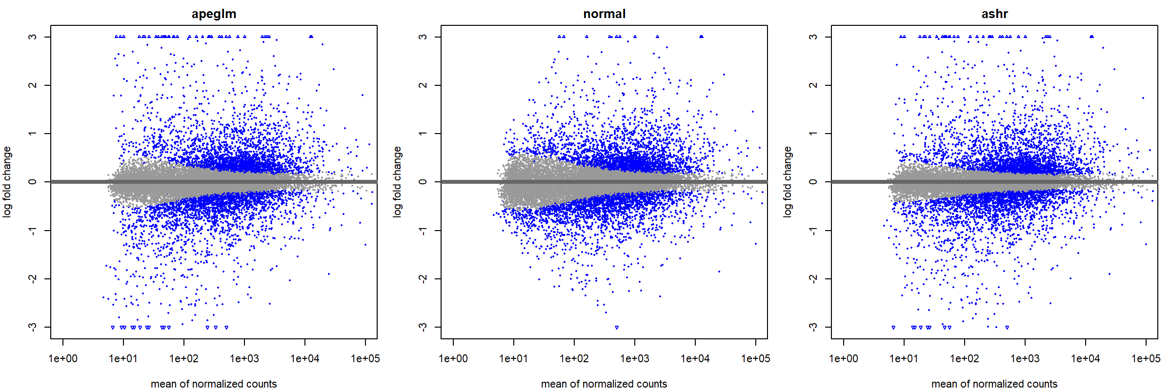
可以使用 lfcThreshold 指定 log2FC 的 Threshold(只需要給正值)
resApeT <- lfcShrink(dds, coef="dex_trt_vs_untrt", type="apeglm", lfcThreshold=1)
png(filename = "./images/MAplot_sig.png", width = 1200, height = 800, res = 200)
plotMA(resApeT, ylim=c(-3,3), cex=.8)
abline(h=c(-1,1), col="dodgerblue", lwd=2)
dev.off()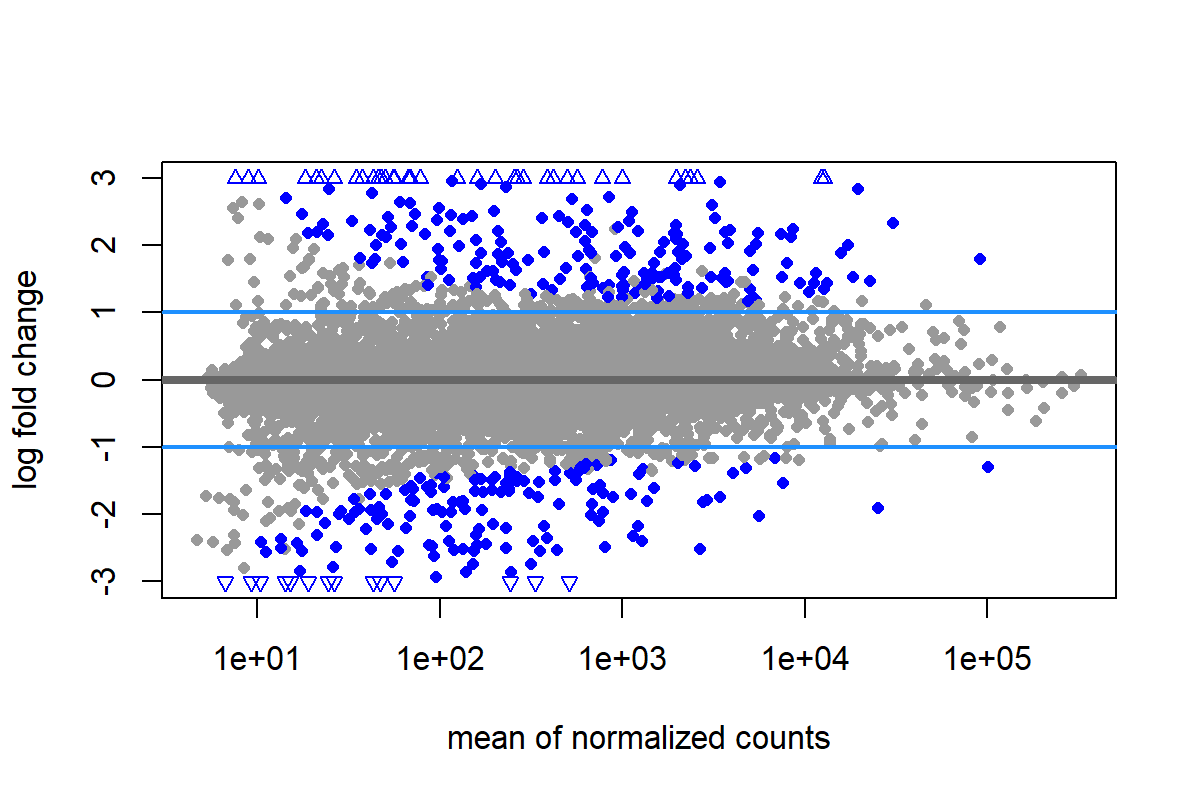
5 匯出到 CSV
write.csv(as.data.frame(resOrdered),
          file="results/deseq2_results.csv")
也可以透過 subset,只選擇輸出顯著結果
resSig <- subset(resOrdered, padj < 0.1)

write.csv(as.data.frame(resSig),
          file="results/deseq2_sig_results.csv")
6 初步結果繪圖
6.1 MA plot
png("./images/MA-plot.png", width = 800, height = 600, res = 120)
plotMA(res, ylim=c(-2,2))
dev.off()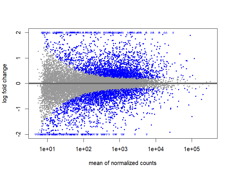
6.2 normalized counts plot
使用 size factor 校正後 的 count 繪製各組別的 count plot
png("./images/count-plot.png", width = 800, height = 600, res = 120)
plotCounts(dds, gene=which.min(res$padj), intgroup="dex")
dev.off()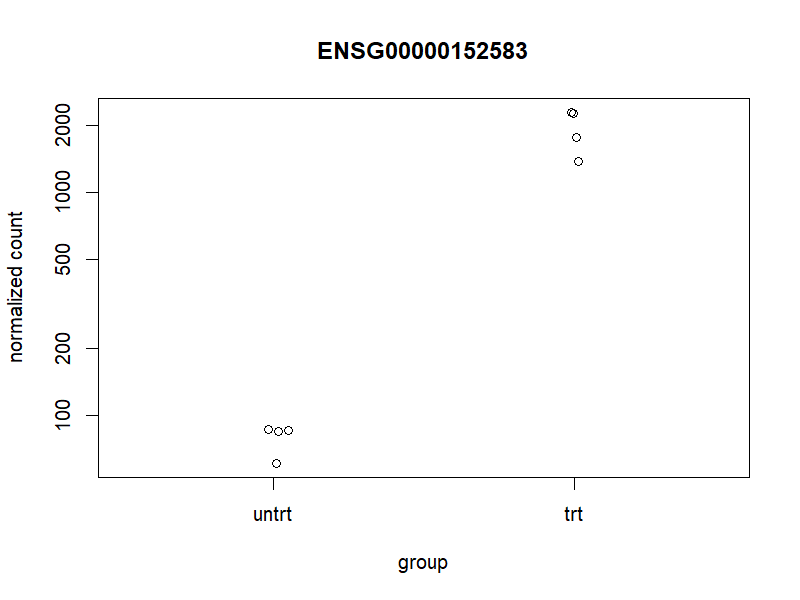
自訂繪圖時,可以使用 returnData=TRUE,輸出可以用於
d <- plotCounts(dds, gene=which.min(res$padj), intgroup="dex",
                returnData=TRUE)
library("ggplot2")
png("./images/count-plot-ggplot.png", width = 800, height = 600, res = 120)
ggplot(d, aes(x=dex, y=count)) +
  geom_point(position=position_jitter(w=0.1,h=0)) +
  scale_y_log10(breaks=c(25,100,400))
dev.off()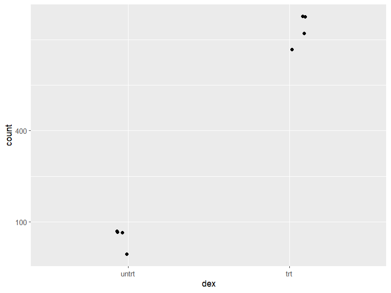
7 對數轉換
對於其他下游分析(例如視覺化或聚類),使用轉換後的計數資料可能更為有效。
Important
DESeq2 在進行差異表達分析時必須使用 raw counts 並透過負二項模型建模;然而在視覺化、分群(PCA、heatmap、clustering)等下游分析中,直接使用 raw counts 或單純取對數(例如 log2(count + pseudocount))的 shifted logarithm 並不理想,因為低表達基因在對數轉換後會產生高度變異。
為此,DESeq2 提供 variance stabilizing transformation (VST) 與 regularized log (rlog) 兩種方法,透過利用整體實驗中「平均表達量與變異數的關係」,將資料轉換為 log2 scale 且變異數較穩定的形式,同時校正 library size 與其他 normalization factors。這兩種轉換的目的不是讓所有基因具有相同變異,而是移除整體的 mean–variance 趨勢,使真正具有生物學差異的基因更容易在樣本分群中被辨識。
vst() 與 rlog() 皆提供 blind 參數,用於控制是否忽略實驗設計資訊。當 blind = TRUE(預設)時,轉換過程不考慮分組資訊,適合用於樣本品質檢查(QC)或探索性分析;但若預期實驗條件會造成大量基因表達差異,建議設為 blind = FALSE,以避免將真實生物學差異誤認為雜訊而過度收縮。實務上,在差異表達分析後進行 PCA 或 heatmap 時,通常建議使用 blind = FALSE。
在樣本數很多(例如數百個樣本)的情況下,rlog() 計算成本較高,vst() 是較有效率且性質相近的替代方案。
# shifted logarithm,this gives log2(n + 1)
ntd <- normTransform(dds)
# variance stabilizing transformation(VST)
vsd <- vst(dds, blind=FALSE)
# regularized log(rlog)
rld <- rlog(dds, blind=FALSE)

head(assay(vsd), 3)
SRR1039508 SRR1039509 SRR1039512 SRR1039513 SRR1039516 SRR1039517 SRR1039520 SRR1039521
ENSG00000000003 9.692790 9.369292 9.825098 9.595346 10.146600 9.833076 9.972598 9.585929
ENSG00000000419 9.269518 9.526153 9.430605 9.468205 9.366965 9.517636 9.264638 9.450769
ENSG00000000457 8.674327 8.603169 8.556368 8.641297 8.492251 8.606475 8.673498 8.629979
Note
下圖比較了三種常見轉換方式(移位對數轉換、正規化對數轉換與變異數穩定變換)在不同表達量範圍內對資料變異的影響。結果顯示,shifted logarithm transformation 在低計數區間會產生較高的標準差,反映其對低表達基因的變異控制能力有限;正規化對數轉換 rlog 可部分緩解此問題,但在低計數區仍保留一定程度的變異放大。相較之下,變異數穩定變換(VST) 能在整個動態範圍內有效平坦化平均值與變異數之間的關係,使不同表達量區間的基因具有更一致的變異結構,因此特別適合用於樣本間比較、分群分析與降維視覺化(如 PCA 與 heatmap)。
library("vsn")
meanSdPlot(assay(ntd))
ggsave("./images/normTransform.png")![]()
meanSdPlot(assay(rld))
ggsave("./images/rld.png")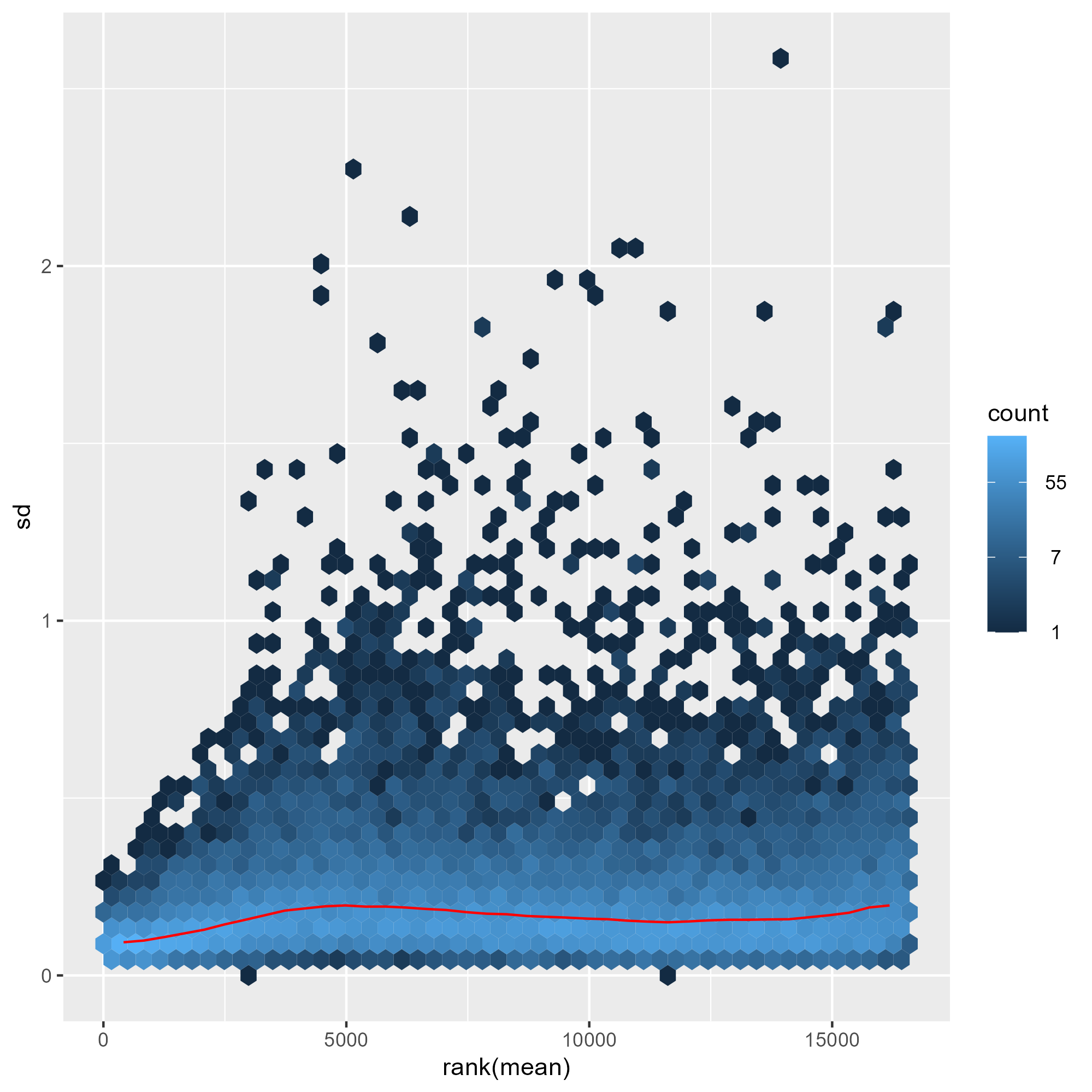
meanSdPlot(assay(vsd))
ggsave("./images/vst.png")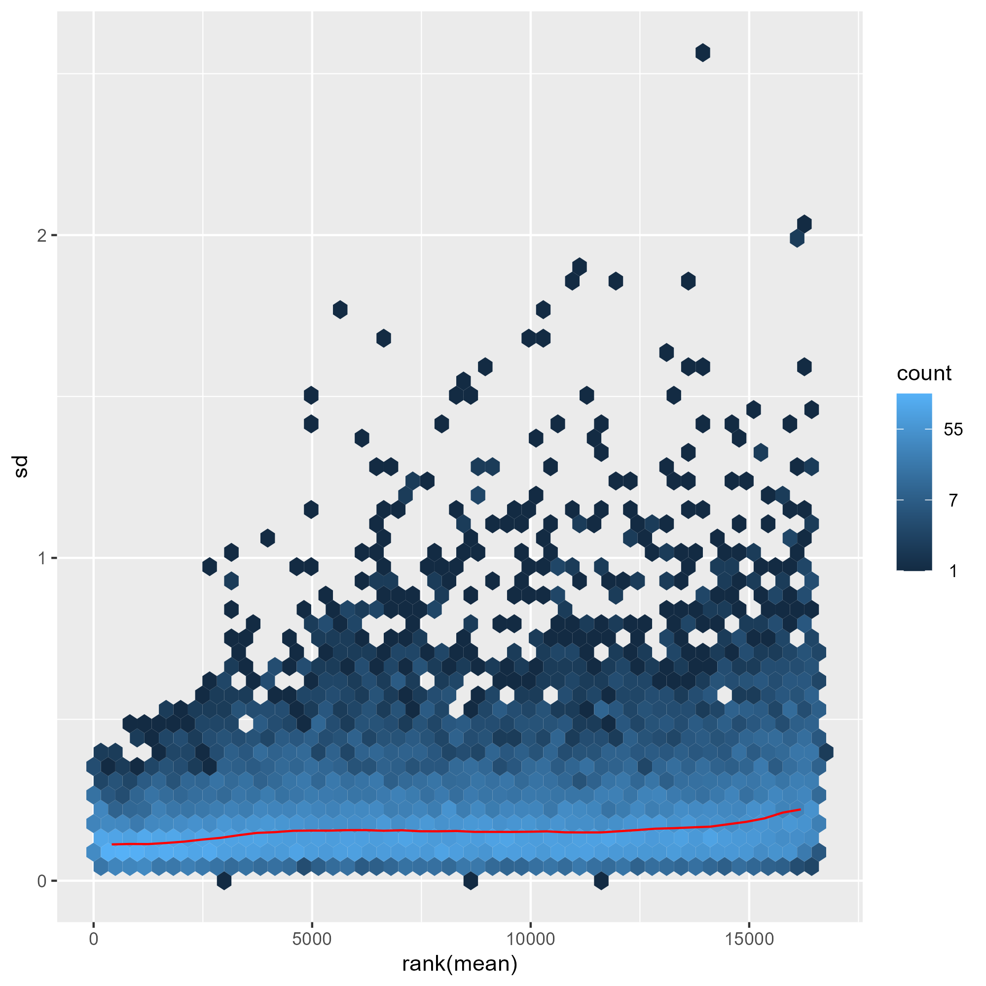
Important
後續建議繪製 heatmap 與 PCA 使用 vst 的結果
8 移除批次效應
Important
本節示範的 batch effect 移除 僅用於 PCA / heatmap 等視覺化用途。
在 DESeq2 中,批次效應應透過設計公式(design,例如 ~ batch + condition)
納入負二項模型中進行校正,而 不應在差異表達分析前手動修改表達矩陣。
# ------------------------------------------------------------
# (示範用)僅用於 PCA 視覺化的 batch effect 移除
# 注意:此步驟不應用於差異表達分析
# ------------------------------------------------------------

# 假設前四個樣本屬於 batch A,後四個樣本屬於 batch B
batch_tmp <- factor(rep(c("A", "B"), each = 4))

# 取出 VST 轉換後的表達矩陣
mat_vst <- assay(vsd)

# 設計矩陣:保留感興趣的生物變數(dex)
design_tmp <- model.matrix(~ dex, colData(vsd))

# 使用 limma 移除 batch effect(僅用於視覺化)
mat_vst_corrected <- limma::removeBatchEffect(
  mat_vst,
  batch  = batch_tmp,
  design = design_tmp
)

# 建立「只用於視覺化」的 vsd 副本
vsd_vis <- vsd
assay(vsd_vis) <- mat_vst_corrected

# PCA 繪圖
plotPCA(vsd_vis, intgroup = c("dex", "cell"))
9 視覺化分析
9.1 heatmap
library("pheatmap")
select <- order(rowMeans(counts(dds,normalized=TRUE)),
                decreasing=TRUE)[1:20]
df <- as.data.frame(colData(dds)[,c("dex","cell")])

png("./images/heatmap.png", width = 800, height = 600, res = 120)
pheatmap(assay(vsd)[select,], cluster_rows=FALSE, show_rownames=FALSE,
         cluster_cols=FALSE, annotation_col=df)
dev.off()
9.2 distance
sampleDists <- dist(t(assay(vsd)))

library("RColorBrewer")
sampleDistMatrix <- as.matrix(sampleDists)
rownames(sampleDistMatrix) <- paste(vsd$dex, vsd$cell, sep="-")
colnames(sampleDistMatrix) <- NULL
colors <- colorRampPalette( rev(brewer.pal(9, "Blues")) )(255)

png("./images/distance.png", width = 800, height = 600, res = 120)
pheatmap(sampleDistMatrix,
         clustering_distance_rows=sampleDists,
         clustering_distance_cols=sampleDists,
         col=colors)
dev.off()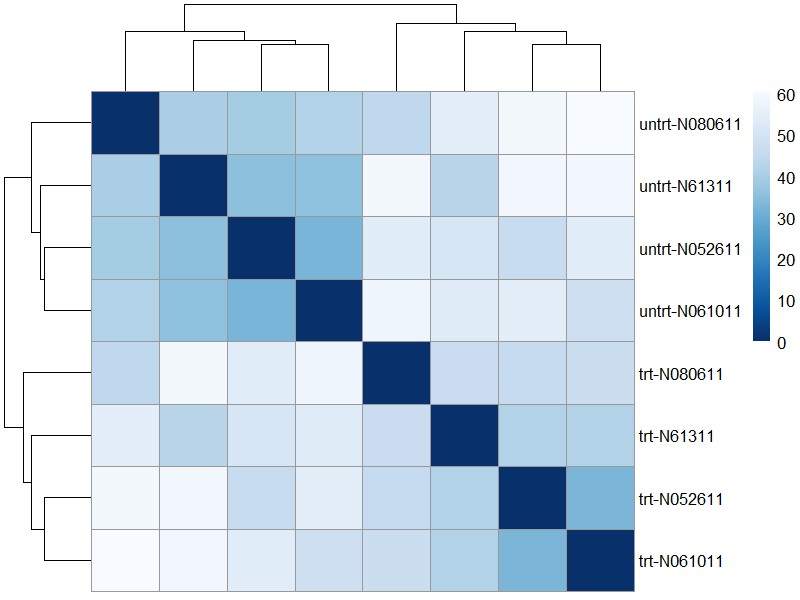
9.3 PCA
png("./images/PCA.png", width = 800, height = 600, res = 120)
plotPCA(vsd, intgroup=c("dex", "cell"))
dev.off()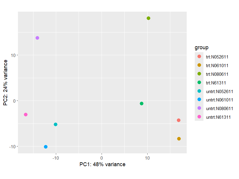
pcaData <- plotPCA(vsd, intgroup=c("dex", "cell"), returnData=TRUE)
percentVar <- round(100 * attr(pcaData, "percentVar"))
ggplot(pcaData, aes(PC1, PC2, color=dex, shape=cell)) +
  geom_point(size=3) +
  xlab(paste0("PC1: ",percentVar[1],"% variance")) +
  ylab(paste0("PC2: ",percentVar[2],"% variance")) +
  coord_fixed()
ggsave("./images/customize-PCA.png")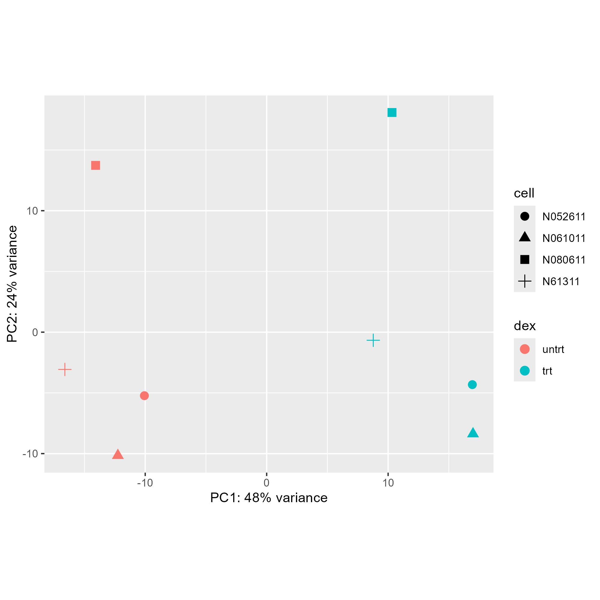
9.4 檢視異常值
png("./images/cooks.png", width = 800, height = 600, res = 120)
par(mar=c(8,5,2,2))
boxplot(log10(assays(dds)[["cooks"]]), range=0, las=2)
dev.off()
par(mfrow = c(1,1))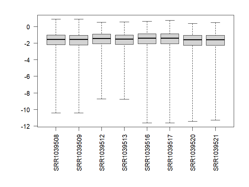
9.5 離散度估計圖
png("./images/dispersions.png", width = 800, height = 600, res = 120)
plotDispEsts(dds)
dev.off()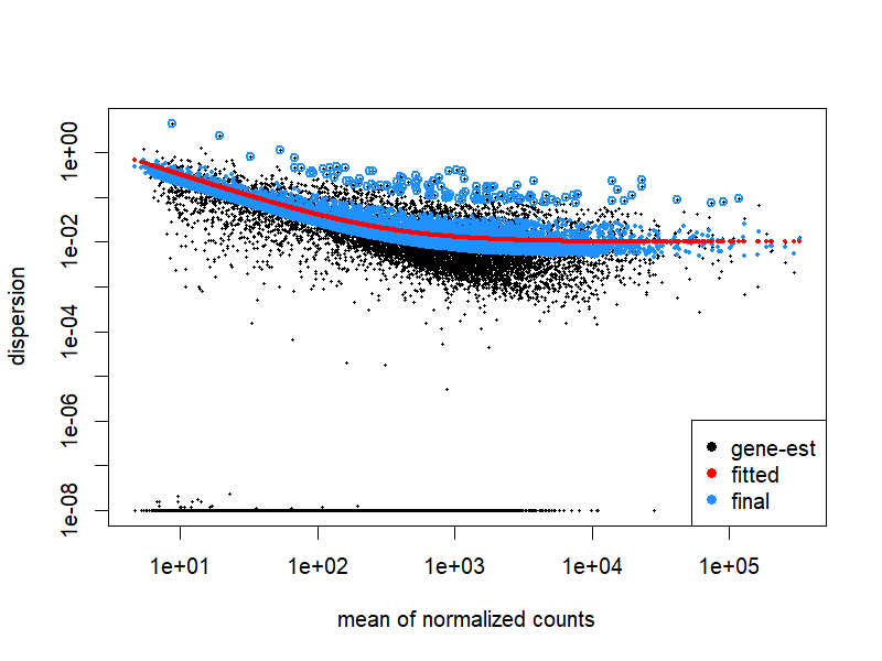
9.6 獨立篩選結果
png("./images/independentFiltering.png", width = 800, height = 600, res = 120)
plot(metadata(res)$filterNumRej,
     type="b", ylab="number of rejections",
     xlab="quantiles of filter")
lines(metadata(res)$lo.fit, col="red")
abline(v=metadata(res)$filterTheta)
dev.off()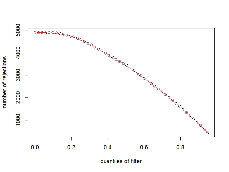
resNoFilt <- results(dds, independentFiltering=FALSE)
addmargins(table(filtering=(res$padj < .1),
                 noFiltering=(resNoFilt$padj < .1)))
noFiltering
filtering FALSE TRUE Sum
FALSE 11680 0 11680
TRUE 0 4916 4916
Sum 11680 4916 165969.7 顯著的 MA plot
png("./images/MA-sig-multi.png", width = 800, height = 600, res = 120)
par(mfrow=c(2,2),mar=c(2,2,1,1))
ylim <- c(-2.5,2.5)
resGA <- results(dds, lfcThreshold=.5, altHypothesis="greaterAbs")
resLA <- results(dds, lfcThreshold=.5, altHypothesis="lessAbs")
resG <- results(dds, lfcThreshold=.5, altHypothesis="greater")
resL <- results(dds, lfcThreshold=.5, altHypothesis="less")
drawLines <- function() abline(h=c(-.5,.5),col="dodgerblue",lwd=2)
plotMA(resGA, ylim=ylim); drawLines()
plotMA(resLA, ylim=ylim); drawLines()
plotMA(resG, ylim=ylim); drawLines()
plotMA(resL, ylim=ylim); drawLines()
dev.off()
par(mfrow = c(1,1))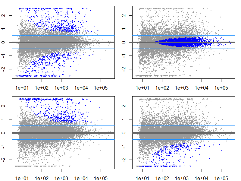
10 索引結果方法
mcols(dds,use.names=TRUE)[1:4,1:4]DataFrame with 4 rows and 4 columns
gene_id gene_name entrezid gene_biotype
<character> <character> <integer> <character>
ENSG00000000003 ENSG00000000003 TSPAN6 NA protein_coding
ENSG00000000419 ENSG00000000419 DPM1 NA protein_coding
ENSG00000000457 ENSG00000000457 SCYL3 NA protein_coding
ENSG00000000460 ENSG00000000460 C1orf112 NA protein_codingsubstr(names(mcols(dds)),1,10) [1] "gene_id" "gene_name" "entrezid" "gene_bioty" "gene_seq_s" "gene_seq_e" "seq_name" "seq_strand" "seq_coord_" "symbol"
[11] "baseMean" "baseVar" "allZero" "dispGeneEs" "dispGeneIt" "dispFit" "dispersion" "dispIter" "dispOutlie" "dispMAP"
[21] "Intercept" "cell_N0610" "cell_N0806" "cell_N6131" "dex_trt_vs" "SE_Interce" "SE_cell_N0" "SE_cell_N0" "SE_cell_N6" "SE_dex_trt"
[31] "WaldStatis" "WaldStatis" "WaldStatis" "WaldStatis" "WaldStatis" "WaldPvalue" "WaldPvalue" "WaldPvalue" "WaldPvalue" "WaldPvalue"
[41] "betaConv" "betaIter" "deviance" "maxCooks" mcols(mcols(dds), use.names=TRUE)[1:4,]DataFrame with 4 rows and 2 columns
type description
<character> <character>
gene_id input
gene_name input
entrezid input
gene_biotype input head(assays(dds)[["mu"]]) SRR1039508 SRR1039509 SRR1039512 SRR1039513 SRR1039516 SRR1039517 SRR1039520 SRR1039521
ENSG00000000003 673.34248 452.08160 902.51831 393.17109 1142.79858 1042.58208 747.83158 590.14459
ENSG00000000419 488.64748 493.18652 590.34452 386.60353 584.75637 801.95544 422.69920 501.44208
ENSG00000000457 247.66005 222.34744 271.65052 158.24553 258.41249 315.24588 224.95803 237.38403
ENSG00000000460 63.38351 52.08835 51.53345 27.47883 67.09037 74.91767 69.08345 66.72862
ENSG00000000971 3190.58151 3749.57917 5877.62169 4481.86794 6813.50109 10880.34732 5483.02959 7573.68242
ENSG00000001036 1434.12090 1061.14400 1782.02739 855.55449 1427.62097 1435.36127 1317.39369 1145.71857head(assays(dds)[["cooks"]]) SRR1039508 SRR1039509 SRR1039512 SRR1039513 SRR1039516 SRR1039517 SRR1039520 SRR1039521
ENSG00000000003 1.616130e-03 1.519961e-03 0.02723217 0.02412281 0.0004105617 0.0004075197 0.01981396 0.019216709
ENSG00000000419 4.115407e-02 4.120745e-02 0.06248341 0.05851166 0.0003087819 0.0003196843 0.00360783 0.003707157
ENSG00000000457 5.169819e-02 5.043213e-02 0.02385542 0.02074311 0.0538511444 0.0559503340 0.02508845 0.025403962
ENSG00000000460 4.213300e-02 3.892083e-02 0.78004483 0.54909816 0.3782274780 0.3927170123 0.14870346 0.146891121
ENSG00000000971 2.852352e-03 2.864018e-03 0.02123342 0.02113580 0.0014944796 0.0015017207 0.02532674 0.025439142
ENSG00000001036 1.387361e-05 1.353068e-05 0.01824741 0.01715301 0.0001420261 0.0001420757 0.02213142 0.021875429head(dispersions(dds))
head(mcols(dds)$dispersion)[1] 0.00826147 0.01002723 0.01490438 0.05677705 0.00748182 0.00693662
[1] 0.00826147 0.01002723 0.01490438 0.05677705 0.00748182 0.00693662sizeFactors(dds)SRR1039508 SRR1039509 SRR1039512 SRR1039513 SRR1039516 SRR1039517 SRR1039520 SRR1039521
1.0223204 0.8956557 1.1751624 0.6680312 1.1760124 1.3999925 0.9169654 0.9442367 head(coef(dds)) Intercept cell_N061011_vs_N052611 cell_N080611_vs_N052611 cell_N61311_vs_N052611 dex_trt_vs_untrt
ENSG00000000003 9.584952 0.08667815 0.33950004 -0.22160289 -0.38392609
ENSG00000000419 8.972553 -0.12400478 -0.01476449 -0.07175025 0.20417051
ENSG00000000457 7.852748 0.08582504 -0.07311903 0.06762217 0.03528580
ENSG00000000460 5.454577 0.78075193 0.37955356 0.49961124 -0.09231568
ENSG00000000971 12.288157 0.25766172 0.21212080 -0.68040028 0.42374050
ENSG00000001036 10.566444 -0.07791200 -0.32094952 -0.11234002 -0.24371500attr(dds, "betaPriorVar")[1] 1e+06 1e+06 1e+06 1e+06 1e+06priorInfo(resLFC) Intercept cell_N061011_vs_N052611 cell_N080611_vs_N052611 cell_N61311_vs_N052611 dex_trt_vs_untrt
ENSG00000000003 9.584952 0.08667815 0.33950004 -0.22160289 -0.38392609
ENSG00000000419 8.972553 -0.12400478 -0.01476449 -0.07175025 0.20417051
ENSG00000000457 7.852748 0.08582504 -0.07311903 0.06762217 0.03528580
ENSG00000000460 5.454577 0.78075193 0.37955356 0.49961124 -0.09231568
ENSG00000000971 12.288157 0.25766172 0.21212080 -0.68040028 0.42374050
ENSG00000001036 10.566444 -0.07791200 -0.32094952 -0.11234002 -0.24371500
> attr(dds, "betaPriorVar")
[1] 1e+06 1e+06 1e+06 1e+06 1e+06
> priorInfo(resLFC)
$type
[1] "apeglm"
$package
[1] "apeglm"
$version
[1] ‘1.28.0’
$prior.control
$prior.control$no.shrink
[1] 1 2 3 4
$prior.control$prior.mean
[1] 0
$prior.control$prior.scale
[1] 0.31093
$prior.control$prior.df
[1] 1
$prior.control$prior.no.shrink.mean
[1] 0
$prior.control$prior.no.shrink.scale
[1] 15
$prior.control$prior.var
[1] 0.09667748priorInfo(resNorm)$type
[1] "normal"
$package
[1] "DESeq2"
$version
[1] ‘1.46.0’
$betaPriorVar
Intercept cellN061011 cellN080611 cellN61311 dextrt
1.000000e+06 9.533906e-02 2.021624e-01 1.735684e-01 2.737881e-01 priorInfo(resAsh)$type
[1] "ashr"
$package
[1] "ashr"
$version
[1] ‘2.2.63’
$fitted_g
$pi
[1] 0.0439744520 0.0000000000 0.0000000000 0.0000000000 0.0685644908 0.0000000000 0.0000000000 0.0000000000 0.0000000000 0.1450487790
[11] 0.4059417499 0.0000000000 0.0638784291 0.2095170944 0.0000000000 0.0307184366 0.0314564441 0.0000000000 0.0003641027 0.0005360216
[21] 0.0000000000 0.0000000000 0.0000000000 0.0000000000
$mean
[1] 0 0 0 0 0 0 0 0 0 0 0 0 0 0 0 0 0 0 0 0 0 0 0 0
$sd
[1] 0.006522069 0.009223599 0.013044138 0.018447197 0.026088277 0.036894395 0.052176554 0.073788790 0.104353107 0.147577580
[11] 0.208706215 0.295155159 0.417412429 0.590310319 0.834824859 1.180620637 1.669649717 2.361241274 3.339299434 4.722482549
[21] 6.678598869 9.444965098 13.357197737 18.889930195
attr(,"class")
[1] "normalmix"
attr(,"row.names")
[1] 1 2 3 4 5 6 7 8 9 10 11 12 13 14 15 16 17 18 19 20 21 22 23 24dispersionFunction(dds)function (q)
coefs[1] + coefs[2]/q
<bytecode: 0x000002b54cccbc00>
<environment: 0x000002b576d03618>
attr(,"coefficients")
asymptDisp extraPois
0.01004404 3.15951336
attr(,"fitType")
[1] "parametric"
attr(,"varLogDispEsts")
[1] 0.9537109
attr(,"dispPriorVar")
[1] 0.5205205attr(dispersionFunction(dds), "dispPriorVar")[1] 0.5205205metadata(dds)[["version"]][1] ‘1.46.0’11 備註
Note
進階議題說明
在部分高度複雜的實驗設計(例如巢狀設計、重複量測或嚴重不平衡設計)中, 可能會遇到模型矩陣未滿秩(non–full rank)的問題, 此時需重新構建設計或手動指定模型矩陣。 本教學聚焦於常見且可穩定擬合的設計情境,相關進階內容可參考 DESeq2 官方文件。
12 其他視覺化軟體
- regionReport
- Glimma
- pcaExplorer
- iSEE/iSEEde
- DEvis
13 建議流程圖
flowchart TD
    A[Raw counts] --> B[DESeqDataSet]
    B --> C[DESeq: size factor, dispersion, NB GLM]
    C --> D[results: log2FC, pvalue, padj]

    D --> E[GSEA using Wald stat]

    C --> F[VST transformed counts]
    F --> G[removeBatchEffect for visualization]
    G --> H[PCA or MDS]
    G --> I[Heatmap]

    D --> J[lfcShrink for effect size]
    J --> K[MA plot or report table]